7 Systems of first order ODEs
In this chapter we study systems of first order ODEs in more detail. Equivalently, we study vector-valued first order ODEs, i.e. the equation \[\dot{z}(t)=F(t,z(t))\] for \(z(t)\in\mathbb{R}^{d}\) or \(z(t)\in\mathbb{C}^{d},\) where the vector-valued function \(F\) takes values in the the same space.
7.1 Direction fields for autonomous planar systems
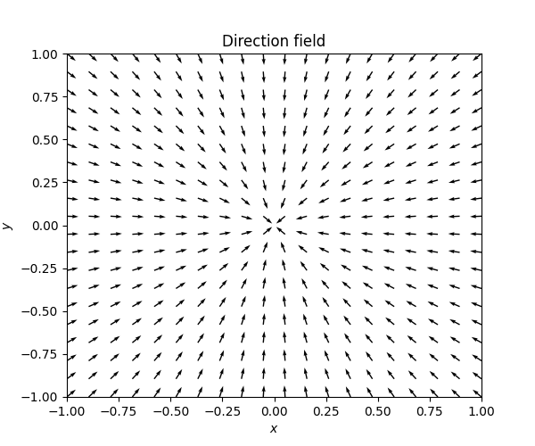
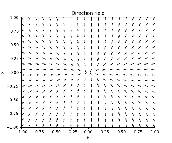
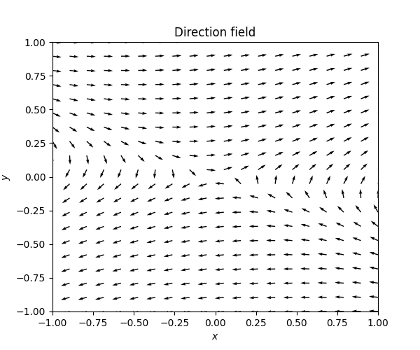
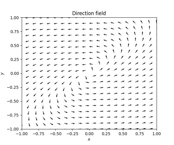
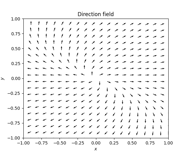
We have often used the tangent fields introduced in Section 3.1 to graphically investigate the solutions of \(\mathbb{R}\)-valued first order ODEs. There is a related graphical technique for first order \(\mathbb{R}^{2}\)-valued autonomous ODEs: the direction field. Consider the ODE \[\dot{z}(t)=F(z(t))\quad\quad\text{for }\quad\quad z(t)=(x(t),y(t))\quad\quad\text{ and }\quad\quad F:A\to\mathbb{R}^{2}\tag{7.1}\] for \(A=\mathbb{R}^{2}\) or a subset thereof. Like the tanget field, the direction field is a collection of arrows showing the direction the solutions take on a grid \((x_{i},y_{i})\) in \(\mathbb{R}^{2}\) - in this case, an arrow in the direction of the vector \(F(x_{i},y_{i}).\) For the ODE \[\dot{z}=\left(\begin{matrix}2xy\\ 1+y^{2}x^{2} \end{matrix}\right)\tag{7.2}\] (where \(z=(x,y)\)) one can draw the following direction field:
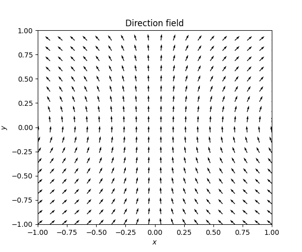
The arrows are drawn with a fixed length, regardless of the magnitude of the vector \(F(x_{i},y_{i}).\) The vector in the direction of \(F(x,y)\) of unit length is \[\frac{F(x,y)}{\left|F(x,y)\right|}=\frac{F(x,y)}{\sqrt{F_{1}(x,y)^{2}+F_{2}(x,y)^{2}}}=\frac{\left(F_{1}(x,y),F_{2}(x,y)\right)}{\sqrt{F_{1}(x,y)^{2}+F_{2}(x,y)^{2}}}.\] This means that one fixes an appropriate length \(l\) and draw a line from \[(x_{i},y_{i})-\frac{l}{2}\frac{F(x_{i},y_{i})}{\left|F(x_{i},y_{i})\right|}\quad\quad\text{ to }\quad\quad(x_{i},y_{i})+\frac{l}{2}\frac{F(x_{i},y_{i})}{\left|F(x_{i},y_{i})\right|}.\] In computer algebra systems or math libraries there are often functions that can help with creating these plots. In Python with mathplotlib and numpy one can use the function “matplotlib.pyplot.quiver”. It automatically picks an approriate size and length of the arrows.
# Make a direction field for the ODE
# x' = x*y*2
# y' = 1 + y**2
import numpy as np import matplotlib.pyplot as plt
# Range of plot
xmin = -1
xmax = 1
ymin = -1
ymax = 1
# Create a vector of evenly spaced values between xmin and xmax
x = np.linspace( xmin, xmax, 20
# Create a vector of evenly spaced values between ymin and ymax
y = np.linspace( ymin, ymax, 20 )
# Turn the x vector into a row vector
xrowvec = x.reshape(1,20) # Turn the y vector into a column vector
ycolvec = y.reshape(20,1 )
# Compute the derivative prescribed by the ODE
# at each point of the grid
dx = np.ones( y.shape + x.shape ) * xrowvec*ycolvec*2
dy = np.ones( y.shape + x.shape ) * (1+ycolvec**2)
# Compute the norms of the derivatives
norms = np.linalg.norm( np.stack( (dx,dy) ), axis = 0 )
# Normalize the derivatives to unit vectors
dx = dx/norms
dy = dy/norms
# Create the plot
plt.figure(figsize=(6, 5))
plt.quiver(x, y, dx, dy, angles='xy')
plt.xlim( xmin, xmax )
plt.ylim( ymin, ymax )
plt.xlabel('$x$')
plt.ylabel('$y$')
plt.title("Direction field")
plt.show()
In Mathematica or Wolfram Alpha one can use the function “StreamPlot”:
StreamPlot[ {x*y*2, 1 + y^2}, {x, -1, 1}, {y, -1, 1}]We sometimes call ODEs of the form ([eq:ch7_planar_ODE]) a planar ODE, since it describes the evolution of a point \(z(t)=(x(t),y(t))\) in the plane \(\mathbb{R}^{2}.\)
Direction field is also an alternative terminology for what we call tangent fields, i.e. the similar diagrams for \(\mathbb{R}\)-valued first order possibly non-autonomous ODEs (Section 3.1). In fact, such an ODE \[\dot{y}(t)=F(t,y(t))\quad\quad\quad\text{ with }\quad\quad\quad y(t)\in\mathbb{R}\tag{7.3}\] can be viewed as a \(\mathbb{R}^{2}\)-valued autonomous ODE for a solution \(z(t)=(y(t),s(t))\in\mathbb{R}^{2},\) by introducing an auxiliary independent variable \(s\) subject to the trivial ODE \[s'(t)=1,\quad\quad\quad s(t_{0})=t_{0},\] so that the solution is simply \(s(t)=t.\) Then the \(\mathbb{R}^{2}\)-valued ODE \[\left(\begin{matrix}\dot{y}(t)\\ \dot{s}(t) \end{matrix}\right)=\tilde{F}(s,y),\quad\quad\text{where}\quad\quad\tilde{F}(s,y)=\left(\begin{matrix}F(s,y)\\ 1 \end{matrix}\right),\tag{7.4}\] is equivalent to ([eq:ch7_note_on_terminology_tangent_field_and_direction_field_fo_ODE]), and the direction field for ([eq:ch7_note_on_terminology_tangent_field_and_direction_field_fo_system]) is exactly the same diagram as the tangent field for ([eq:ch7_note_on_terminology_tangent_field_and_direction_field_fo_ODE]).
7.2 Planar phase portraits
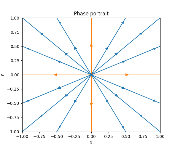
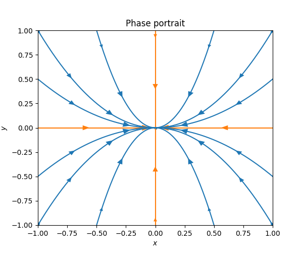
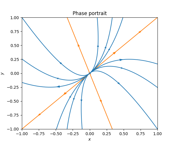
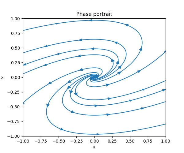
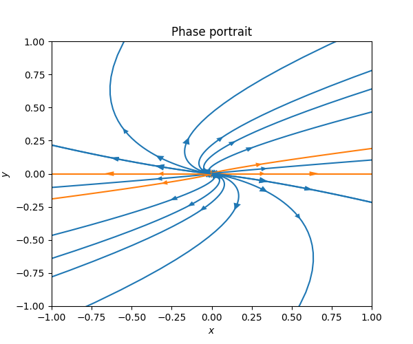
A related but different way to visualize the solutions to a planar ODE is with a phase portrait, also known as a phase diagram. The phase portrait consists of some representative solution curves, together with arrows indicating the direction of the solution as it moves along the curve. For the ODE ([eq:ch7_direction_field_first_example]) one can draw the following phase portrait. It allows one to quickly grasp - or concisely express - the different qualitative behaviors that are present in the solutions of the ODE.
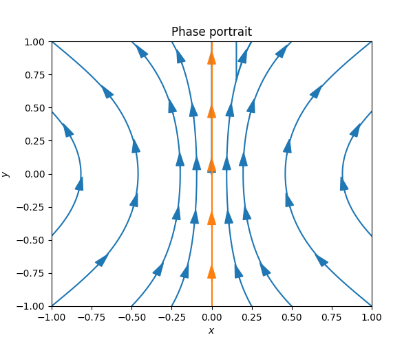
Cf. the direction field of the same ODE in Figure Figure 7.1.
This phase portrait was drawn on a computer with exact solution curves, but one can also draw approximate but qualitatively informative phase portraits by pen and paper.
Indeed the qualitative picture in Figure Figure 7.2 can be derived directly from the equation ([eq:ch7_direction_field_first_example]) - the direction field like in Figure Figure 7.1 is helpful but not necessary. Since \(1+y^{2}x^{2}\ge1\) for all \(x,y\) the solution curves always move upwards. Since the sign of \(2xy\) is negative in the lower right-quadrant \(x\ge0,y\le0,\) the solution curves moves towards the \(y\)-axis there. Similarly the solution curves move towards the \(y\)-axis in the bottom-left quadrant \(x\le0,y\le0,\) and away from the \(y\)-axis for \(y\ge0.\)
The orange curve in the middle is special: it is a solution whose \(x\) coordinate does not change with \(t.\) Indeed if \(z(t)=(0,t)\) then since \[\dot{x}=0=2xy\checkmark\quad\quad\text{ and }\quad\quad\dot{y}=1=1+x^{2}y^{2}\checkmark,\] so \(z(t)=(0,t)\) is a solution. This solution is also a boundary between two types of behaviors: solutions to the left of it move left for \(y\le0,\) and then right for \(y\ge0,\) while solutions to the right of it move first right and then left. It is common to include such boundary solutions, which partition the plane into regions of qualitatively different behavior, in phase portraits.
7.3 Phase portraits and direction fields for second order autonomous ODEs
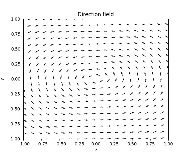
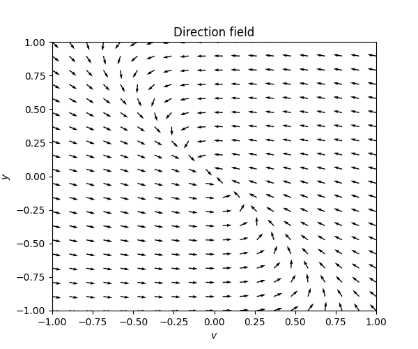
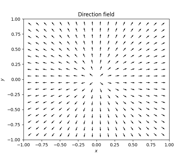
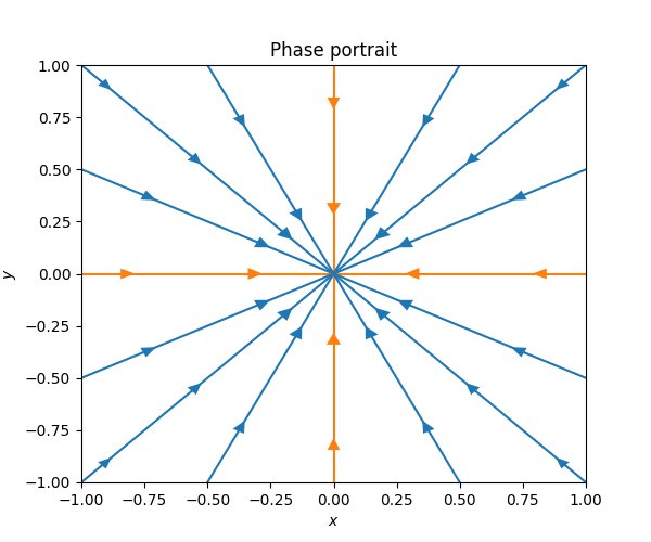
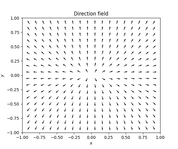
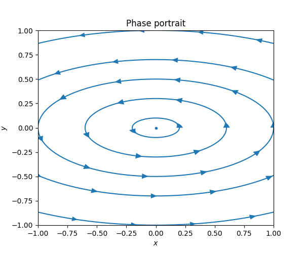
These diagrams can also be used to graphically investigate the solutions of a second order autonomous ODE, by turning the second order ODE into a system of two first-order ODEs, as we did in Section 6.2. Let us plot the solutions of the harmonic oscillator from Section 5.2 in this way. The equation is \[\ddot{y}+\gamma\dot{y}+ky=0,\] for \(k>0,\gamma\ge0.\) With the change of variables \(v=\dot{y}\) (\(v\) for velocity), so that \(\ddot{y}=v,\) we obtain the corresponding \(\mathbb{R}^{2}\)-valued first order ODE \[{\dot{v} \choose \dot{y}}={-\gamma v-ky \choose v}.\] \(\text{ }\) Undamped Let us consider the undamped case \(\gamma=0.\) Then the equation simplifies to \[{\dot{y} \choose \dot{v}}={v \choose -ky}.\tag{7.5}\] The next figure shows the direction field for this ODE with \(k=2.\)
It looks like the solutions plotted in the \((v,y)\)-plane rotate around the origin \((v,y)=0.\) Recall the general undamped solution \[y=\alpha\cos(\sqrt{k}t+s)\] from ([eq:ch5_aut_spring_mass_undamped_gen_sol]). Taking the derivative to compute \(v\) we obtain \[v=-\sqrt{k}\alpha\sin(\sqrt{k}t+s).\] The corresponding solution to ([eq:ch7_harm_osc_as_sys_undamped_ode]) is \[\left(\begin{matrix}v\\ y \end{matrix}\right)=\alpha\left(\begin{matrix}-\sin(\sqrt{k}t+s)\sqrt{k}\\ \cos(\sqrt{k}t+s) \end{matrix}\right),\] which is the parametric form of an ellipse centered at \((0,0)\)! Plotting the solutions corresponding to \(\alpha\in\{0.1,0.25,0.5,0.75,1.0\}\) we obtain the following phase portrait
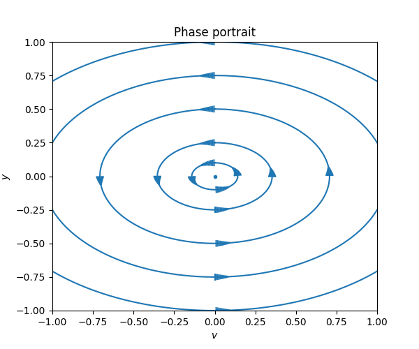
The dot in the middle represents the stationary solution \((v,y)=0,t\ge0.\) Several important properties of the undamped harmonic oscillator are reflected in this phase portrait:
The solutions are periodic, which is the reason that each solution is a closed curve.
The solution curves are the ellipses defined by \(y^{2}k+v^{2}=\alpha^{2}k.\) This means that for each solution the quantity \[y(t)^{2}k+v(t)^{2}\tag{7.7}\] is constant in time.
Point 2 corresponds to an important physical principle: conservation of energy. Since this is a model of an idealized undamped oscillator, no energy is lost as the system evolves. The energy of the system consists of the kinetic energy of the weight, which is given by \(\frac{1}{2}v^{2}\) (for \(m=1\)), and the potential energy stored in the spring when it is compressed or pulled away from \(y=0,\) which is \(\frac{1}{2}ky^{2}.\) Thus the total energy is \[\frac{y(t)^{2}k+v(t)^{2}}{2},\] which is if course simply ([eq:ch6_undamped_convervation_of_energy]) divided by \(2,\) and is therefore indeed constant for each solution.
As the solution evolves energy is converted back and forth between its kinetic and potential forms, with maximal potential energy and minimal (in fact zero) kinetic energy when the solution curves in Figure Figure 7.4 crosses the axis \(v=0,\) and maximal kinetic energy and minimal potential energy when they cross the axis \(y=0.\)
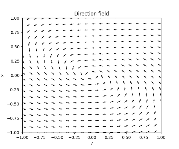
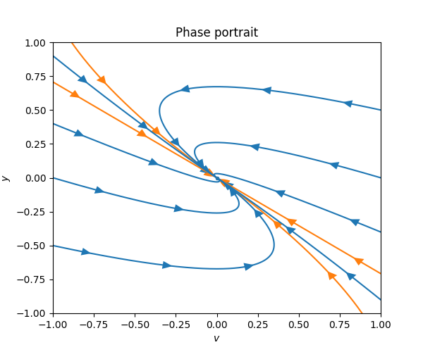
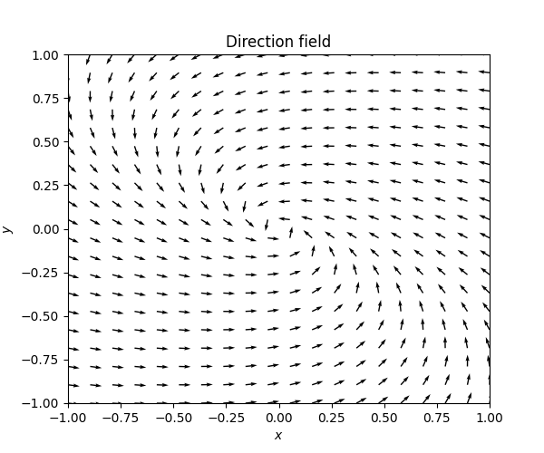
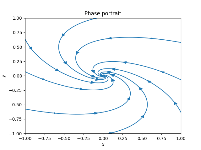
\(\text{ }\) Underdamped The model with a positive friction coefficient \(\gamma>0\) the ODE reads \[{\dot{y} \choose \dot{v}}={v \choose -\gamma v-ky}.\tag{7.8}\] Recall that \(0<\gamma<\sqrt{2}k\) corresponds to an underdamped system, and recall from ([eq:ch5_aut_spring_mass_underdamped_gen_sol]) that the solutions take the form \[y(t)=\alpha e^{-\frac{\gamma}{2}t}\cos(\omega t+s))\quad\quad\quad\text{ for }\quad\quad\quad\omega=\frac{1}{2}\sqrt{4k-\gamma^{2}}\] in this case. The derivative is \[\begin{array}{ccccl} v & = & \dot{y} & = & -\frac{\gamma}{2}e^{-\frac{\gamma}{2}t}\left\{ \alpha\cos(\omega t+s)\right\} +e^{-\frac{\gamma}{2}t}\left\{ -\alpha\omega\sin(\omega t+s)\right\} \\ & & & = & e^{-\frac{\gamma}{2}t}\left\{ -\alpha\frac{\gamma}{2}\cos(\omega t+s)-\alpha\omega\sin(\omega t+s)\right\} . \end{array}\] so the solutions to ([eq:ch7_harm_osc_as_sys_underdamped_ode]) take the form \[\left(\begin{matrix}v\\ y \end{matrix}\right)=\alpha e^{-\frac{\gamma}{2}t}\left(\begin{matrix}-\frac{\gamma}{2}\cos(\omega t+s)-\omega\sin(\omega t+s)\\ \cos(\omega t+s) \end{matrix}\right).\] This formula for different \(\alpha\) can be used to draw a phase portrait for this ODE around the point \((v,y)=0.\) The next figure contains the direction field and the phase portrait.
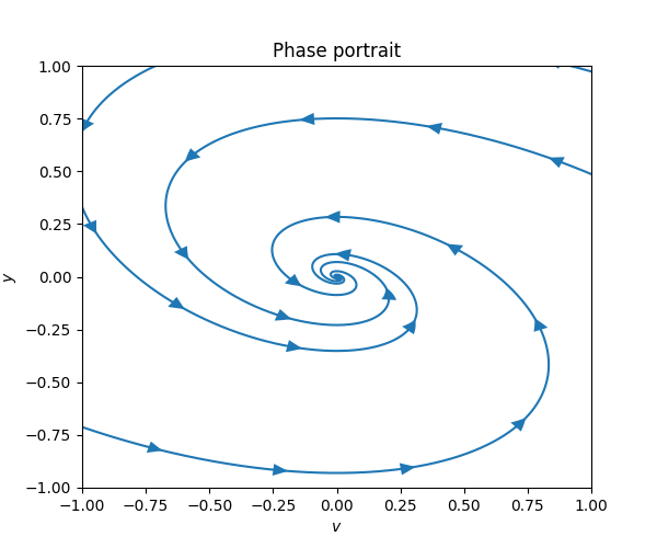
In this phase portrait the solution curve spirals in towards the stationary solution \((v,y)=0.\) The circular motion reflects that energy is still transitioning back and forth between kinetic and potential energy, while the spiraling towards the origin reflects that energy is being lost with each revolution because of the friction.
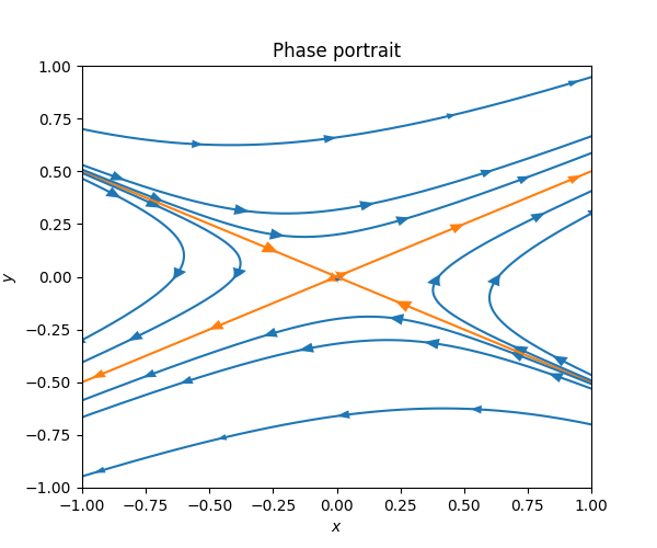
\(\text{ }\) Overdamped For \(\gamma>\sqrt{2}k\) the system is over-damped, and recall from ([eq:ch5_aut_spring_mass_overdamped_gen_sol]) that the solutions take the form \[y(t)=\alpha e^{-\left(\frac{\gamma}{2}+a\right)t}+\beta e^{-\left(\frac{\gamma}{2}-a\right)t},\] for \[a=\frac{1}{2}\sqrt{\gamma^{2}-4k}.\] Taking the derivative we obtain \[v(t)=\dot{y}(t)=-\alpha\left(\frac{\gamma}{2}+a\right)e^{-\left(\frac{\gamma}{2}+a\right)t}-\beta\left(\frac{\gamma}{2}-a\right)e^{-\left(\frac{\gamma}{2}-a\right)t}.\]

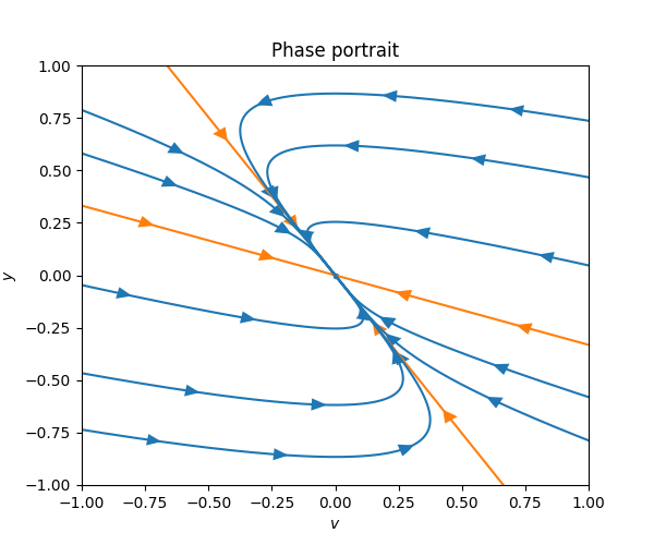
Here we have boundary solutions in orange corresponding to \(\alpha=0\) and \(\beta=0,\) which are solutions that move along straight lines in the phase portrait, and converge on \((v,y)=0.\) These split the phase portrait into four regions. The solutions in the top left and bottom right regions don’t move in a straight line, but do approach the origin \((v,y)=0\) monotonically, without changing directions. The regions to the top right and bottom left by contrast contain solutions that change direction along the \(v\)-axis exactly once before converging on \((v,y)=0.\) This corresponds to solutions where the spring starts with enough energy that it crosses from a compressed to an extended state once before converging.
\(\text{ }\) Critically damped For \(\gamma=\sqrt{2}k\) the system is critically damped, and we recall from ([eq:ch5_aut_spring_mass_crit_damped_gen_sol]) that the solutions take the form \[y(t)=p(t)e^{-\frac{\gamma}{2}t}\] for any first-degree polynomial \(p(t)=\alpha+\beta t.\) The derivative is \[v(t)=\dot{y}(t)=\left\{ p'(t)-\frac{\gamma}{2}p(t)\right\} e^{-\frac{\gamma}{2}t}.\]
In this case one of the boundary solutions is not a straight line, it rather corresponds to the solution \(y(t)=te^{-\frac{\gamma}{2}t}.\) The boundaries split the phase portrait into regions with the same qualitative behavior as in the overdamped case.
7.4 Linear autonomous planar ODEs
In this section we investigate linear autonomous \(\mathbb{R}^{2}\)- or \(\mathbb{C}^{2}\)-valued ODE and associated phase portraits. These ODEs have the form \[\dot{z}=Az+b\tag{7.12}\] for \(z=(x,y)\in\mathbb{R}^{2}\text{ or }\mathbb{C}^{2},\) where \(A\) is a constant a matrix and \(b\) a constant vector.
\(\text{ }\) Stationary solution. Firstly, we note that under the additional assumption that \(A\) is invertible we can set \[z_{*}=-A^{-1}b,\] and then \[z(t)=z_{*}\quad\quad\quad\forall t\] is a stationary solution to the ODE, since \(\dot{z}=0\) and \[Az(t)+b=Az_{*}+b=A\left(-A^{-1}b\right)+b=-b+b=0.\]
Furthermore a function \(u(t)\) solves ([eq:ch7_lin_aut_plan_lin_general_form]) iff \(z(t)=u(t)-z_{*}\) solves the homogeneous ODE \[\dot{z}=Az.\tag{7.13}\] We thus focus on ([eq:ch7_lin_aut_plan_lin_homo_general_form]).
(Complete solution of first order autonomous ODEs with \(a\ne0\)). Assume \(a,b\in\mathbb{R},a\ne0\) and \(I\subset\mathbb{R}\) an interval. Then a function \(y(t)\) is a solution of the ODE \[\dot{y}(t)=ay(t)+b,\quad\quad t\in I,\tag{3.23}\] iff \[y(t)=\alpha e^{at}-\frac{b}{a}\quad\forall t\in I,\text{ for some }\alpha\in\mathbb{R}.\tag{3.24}\]
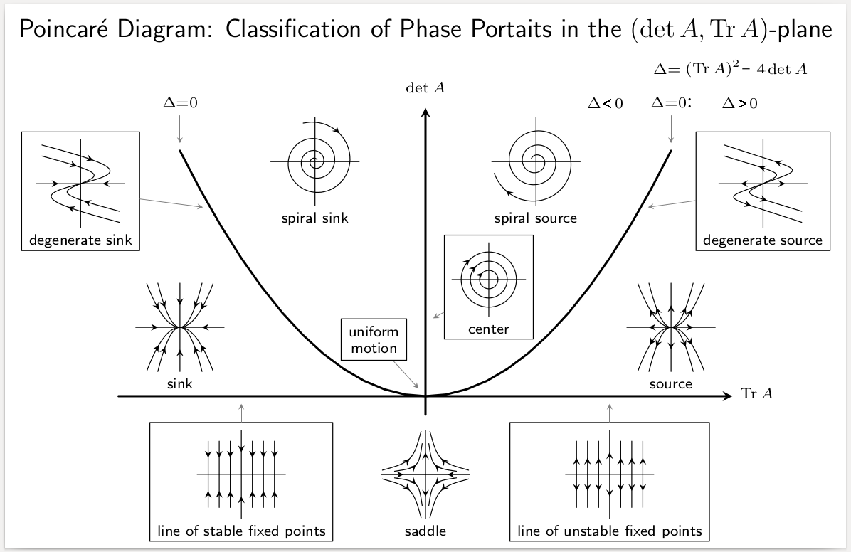
An equilibrium point which has solution curves leading into it from all sides, like Figure Figure 7.9 and Figure Figure 7.11, is called a sink. An equilibrium point that only has solution curves leaving it, like in Figure Figure 7.8 and Figure Figure 7.12, is called a source. The overdamped harmonic spring in Figure Figure 7.6 is another example of a sink.
A previous version of this chapter had an invalid argument for the following incorrect claim: For any \(A\in\mathbb{C}^{2\times2},\) if \(z\) is a solution of \(z=Az\) and \(v\) is an eigenvector \(v\) of \(A\) when eigenvalue \(\lambda\) then the projection \(z(t)\cdot v\) of \(z(t)\) onto \(v\) satisfies \(z(t)\cdot v=ce^{t\lambda}\) for some constant \(c.\) This is correct only under the additional assumption that \(\lambda\) is not a repeated eigenvalue. If \(\lambda\) is a repeated eigenvalue then \(z(t)\cdot v\) can take the more general form \((c_{1}+tc_{2})e^{t\lambda}.\)
If \(A\) has two distinct real eigenvalues \(\lambda_{1}\ne\lambda_{2},\) then it has two corresponding real eigenvectors \(v_{1},v_{2}\) then \(v_{1}e^{\lambda_{1}t}\) and \(v_{2}e^{\lambda_{2}t}\) are solutions and any linear combination \(a_{1}v_{1}e^{\lambda_{1}t}+a_{2}v_{2}e^{\lambda_{2}t}\) is a solution. Then if \(z(t)\) is any solution there are \(a_{1},a_{2}\) such that \(a_{1}v_{1}+a_{2}v_{2}=z(0)\) (since \(v_{1}\) and \(v_{2}\) are linearly independent), and then \(a_{1}v_{1}e^{\lambda_{1}t}+a_{2}v_{2}e^{\lambda_{2}t}-z(t)\) solves the ODE \(\dot{z}=0,z(0)=0.\) Thus in fact \(z(t)=0\) for all \(t\ge0.\) This proves that \(z\) solves ([eq:ch7_lin_aut_plan_lin_homo_general_form]) iff \(z(t)\cdot v_{1}=c_{1}e^{\lambda_{1}t}\) and \(z(t)\cdot v_{2}=c_{1}e^{\lambda_{2}t},\) when \(\lambda_{1}\ne\lambda_{2}.\) Thus in this case the general solution to ([eq:ch7_lin_aut_plan_lin_homo_general_form]) can be written as \[z(t)=c_{1}v_{1}e^{\lambda_{1}t}+c_{2}v_{2}e^{\lambda_{2}t}.\] An alternative way to view this situation: note that if \(A\) has two distinct real eigenvalues then it is diagonalizable, that is there is an invertible real matrix \(V\) and a diagonal real matrix \(\Lambda\) such that \[A=V^{-1}\Lambda V.\] The matrix \(V\) in fact has the eigenvectors in its columns. By multiplying by \(V^{-1}\) and \(V\) in ([eq:ch7_lin_aut_plan_lin_homo_general_form]) one sees that a solution \(z\) solves ([eq:ch7_lin_aut_plan_lin_homo_general_form]) iff \[\tilde{z}(t)=V^{-1}z(t),\] is a solution of \[\dot{\tilde{z}}(t)=\Lambda\tilde{z}(t).\] One can also argue more abstractly but faster by noting that if \(A\) is diagonalizable there is a basis where it equals the diagonal matrix \(\Lambda,\) and the ODE ([eq:ch7_lin_aut_plan_lin_homo_general_form]) written in this basis is \[\dot{z}(t)=\Lambda z(t).\] Thus the the ODE ([eq:ch7_lin_aut_plan_lin_homo_general_form]) with two real eigenvalues is up to a change of basis equivalent to the diagonal case ([eq:ch7_lin_aut_plan_lin_homo_diagonal])-([eq:ch7_lin_aut_plan_lin_homo_diagonal_ODE]). The phase portraits look qualitatively the same, up to the change of basis.
For instance, consider
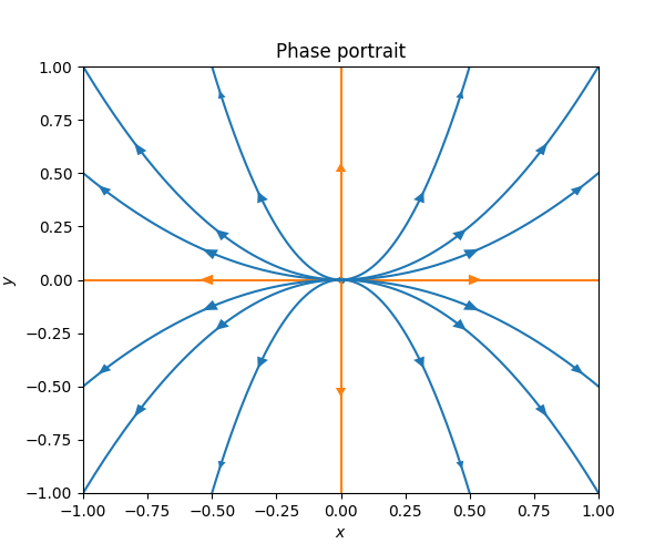
\[\dot{z}=Az\quad\quad\quad\quad A=\left(\begin{matrix}5 & -1\\ -3 & 7 \end{matrix}\right).\tag{7.17}\] This \(A\) has eigenvectors \[v_{1}=\left(\begin{matrix}1\\ 1 \end{matrix}\right),\quad\quad v_{2}=\left(\begin{matrix}\frac{1}{3}\\ -1 \end{matrix}\right),\] and eigenvalues \[\lambda_{1}=4\quad\quad\lambda_{2}=8.\] The direction field and phase portrait of this ODE look as follows.
Note that with the terminology introduced above this is a source.
Next consider the ODE \[\dot{z}=Az\quad\quad\quad\quad\text{for}\quad\quad\quad\quad A=\left(\begin{matrix}\frac{1}{2} & 3\\ \frac{3}{4} & \frac{1}{2} \end{matrix}\right),\tag{7.19}\] whose \(A\) has eigenvectors \[v_{1}=\left(\begin{matrix}2\\ 1 \end{matrix}\right),\quad\quad v_{2}=\left(\begin{matrix}2\\ -1 \end{matrix}\right),\] and eigenvalues \[\lambda_{1}=2,\quad\quad\lambda_{2}=-1.\] The phase portrait looks as follows.
An equilibrium point like this which has both solution curves converging to it and other solution curves moving away from is called a saddle point. Only the two orange curves with arrows pointing towards the equilibrium points actually converge to it. Any perturbation away from these thin curves, however small, leads to a solution which may get close to the equilibrium point, but ultimately escapes it along trajectories like those shown in blue above in Figure Figure 7.13.
\(\text{ }\) Complex linear first order systems. For a complex matrix \(A\) and the corresponding ODE \[\dot{z}=Az,\] the same considerations as for distinct real eigenvalues above imply that for any eigenvector \(v\) and associated eigenvalue \(\lambda\) the complex function \(z(t)=ve^{\lambda t}\) is a solution. These solutions are not easily visualizable with a phase portrait, since four numbers (real and imaginary part of both components) are needed to fully describe the state of the system.
\(\text{ }\) Real matrix with complex eigenvalues. A \(2\times2\) real matrix \(A\) either has only real eigenvalues, or two distinct complex eigenvalues \(\lambda_{1},\lambda_{2},\) which must then satisfy \[\lambda_{1}=\overline{\lambda}_{2},\quad\quad\text{ Im}(\lambda_{1})>0,\] (since they are roots of the real-valued characteristic polynomial). Furthermore the corresponding eigenvectors \(v_{1},v_{2}\) satisfy \[v_{2}=\overline{v}_{1},\] where \(\text{\ensuremath{\overline{\cdot}}}\) denotes component-wise complex conjugation. Thus for such an \(A\) the ODE \[\dot{z}=Az,\tag{7.21}\] has the complex solutions of the form \[\alpha v_{1}e^{\lambda_{1}t}+\beta v_{2}e^{\lambda_{2}t}=\alpha v_{1}e^{rt+\omega t}+\beta\overline{v}_{1}e^{rt-\omega t}\] for any \(\alpha,\beta\in\mathbb{C},\) where \[\lambda_{1}=rt+\omega i\quad\quad\quad\lambda_{2}=rt-\omega i.\] The real solutions in this situation can be written as \[\begin{array}{l} \alpha\frac{ve^{rt+i\omega t}+\overline{v}e^{rt-i\omega t}}{2}+\beta\frac{ve^{rt+i\omega t}-\overline{v}e^{rt-i\omega t}}{2i}=\alpha\mathrm{Re}\left(ve^{rt+i\omega t}\right)+\beta\mathrm{Im}\left(ve^{rt+i\omega t}\right)\end{array}\] for any \(a,b\in\mathbb{R}.\) We can assume w.l.o.g. that \(v_{1}=1,\) and letting \(v_{2}=\rho e^{\theta}\) we then have \[\alpha\frac{ve^{rt+i\omega t}+\overline{v}e^{rt-i\omega t}}{2}+\beta\frac{ve^{rt+i\omega t}-\overline{v}e^{rt-i\omega t}}{2i}=e^{rt}\left\{ \alpha\frac{\cos\left(\omega t+\theta\right)}{2}+\beta\frac{\sin\left(\omega t-\theta\right)}{2i}\right\} .\] The expression \[\alpha\frac{\cos\left(\omega t+\theta\right)}{2}+\beta\frac{\sin\left(\omega t-\theta\right)}{2i}\] is a parametric equation for an ellipse. Thus these are oscillating solutions which move in a ellipse, with growing radius if \(r=\mathrm{Re}\lambda_{1}>0,\) shrinking radius if \(r=\mathrm{Re}\lambda_{1}<0,\) and in a periodic elliptical orbit if \(\mathrm{Re}\lambda_{1}=0.\)
The next diagrams shows a situation where \(\mathrm{Re}\lambda_{1}=0.\)

Such an equilibrium point around which there are periodic solutions that neither decay nor explode is called a center. The harmonic oscillator in the undamped case from Figure Figure 7.4 is another example of a center.
The next diagram shows a situation where \(\mathrm{Re}\lambda_{1}>0.\)
An equilibrium point like in the diagram above is called a spiral source.
The next diagram shows a situation where \(\mathrm{Re}\lambda_{1}<0.\)
An equilibrium point like in the diagram above is called a spiral sink.
\(\text{ }\) Repeated eigenvalue. If a matrix is not diagonalizable, then at least it is similar to matrix in Jordan normal form. For a \(2\times2\) real matrix this means that it is similar to the matrix \[A=\left(\begin{matrix}\lambda & 1\\ 0 & \lambda \end{matrix}\right)\] for some \(\lambda.\) Such a matrix has only one eigenvalue, namely \(v_{1}=\left(\begin{matrix}1\\ 0 \end{matrix}\right).\) Thus \(v_{1}e^{\lambda t}\) is a solution in this case. But there is an additional solution: \[z(t)=\left(\begin{matrix}t\\ 1 \end{matrix}\right)e^{\lambda t}.\] This can be verified by noting that \[\dot{z}(t)=\left(\begin{matrix}1\\ 0 \end{matrix}\right)e^{\lambda t}+\lambda\left(\begin{matrix}t\\ 1 \end{matrix}\right)e^{\lambda t},\] and \[A\left(\begin{matrix}t\\ 1 \end{matrix}\right)e^{\lambda t}=\left(\begin{matrix}\lambda t+1\\ \lambda1 \end{matrix}\right)e^{\lambda t}.\] The next diagram shows such a situation.
We call such a equilibrium point a degenerate source. The harmonic oscillator in Figure Figure 7.7 is an example of degenerate sink.
7.5 Phase portraits of non-linear planar ODEs
The study of phase portraits for non-linear ODEs is part of an area known as dynamical systems. Chaotic dynamical systems are a particularly fascinating subclass. These areas are beyond the scope of this course. In this section we give a brief teaser. If it piques your interest you can read more, for instance in the accessible book “Differential Equations, Dynamical Systems & An Introduction to Chaos” by Hirsch, Smale and Devaney.
Often the most salient features of the solutions of an ODE can be seen around equilibrium points. The linear autonomous planar ODEs from the previous section have a unique equilibrium point, and we cataloged every possible behavior of the solution close to this equilibrium point. Non-linear ODEs may have several critical points. Consider for instance the planar ODE which has equilibrium points at \[x=-1,y=1,\quad\quad x=y=0,\quad\quad x=2,y=0,\quad\quad x=2,y=1.\] The next plot shows a direction field for this ODE. The red “X”-s are the locations of the equilibrium points.
Let us zoom in on the equilibrium points:
We see that this stationary solution is a saddle point, and its behavior looks qualitatively similar to the saddle points of the autonomous linear planar ODEs of the last section. This is obvious from visual inspection. One can confirm it by looking at the Jacobian at the equilibrium point, that is the matrix of derivatives \[J_{F}=\left(\begin{matrix}\partial_{x}F_{1} & \partial_{y}F_{1}\\ \partial_{x}F_{2} & \partial_{y}F_{2} \end{matrix}\right).\] For this equilibrium the Jacobian is \[\left(\begin{matrix}2 & 0\\ 0 & -1 \end{matrix}\right)\] which has a positive and a negative eigenvalue, just like the matrices \(A\) of the planar linear ODEs that featured saddle points in the previous section. The Jacobian of the linear autonomous planar ODEs of the previous section is in fact the matrix \(A\) itself. If the function \(F\) is regular enough it is reasonable to approximate it in the neighborhood of a points \(p\) by the Taylor expansion \[F(p+\Delta)\approx F(p)+\left(J_{F}|_{p}\right)\Delta+\text{lower order terms}.\] For an equilibrium point \(p\) the first term \(F(p)\) vanishes, and the leading order term \(\left(J_{F}|_{p}\right)\Delta\) is exactly the r.h.s. from the corresponding linear autonomous planar ODE. From this point of view it is natural to approximate the ODE ([eq:ch7_dyn_sys_teaser_ODE]) in the neighborhood of this equilibrium by the planar autonomous ODE \[\left(\begin{matrix}\dot{x}\\ \dot{y} \end{matrix}\right)=\left(\begin{matrix}2 & 0\\ 0 & -1 \end{matrix}\right)\left(\begin{matrix}x\\ y \end{matrix}\right).\] An important facet of the theory of dynamical systems is determining when such an approximation by a linear autonomous ODEs is valid, and what kind of behaviors are possible beyond the ones seen in linear autonomous ODEs (some teasers below).
Next we zoom in around the equilibrium point at \((2,0\)).
Visual inspection allows us to classify it as a sink , and again it shows the same qualitative behavior as the sinks of the linear planar ODEs of the last section. The Jacobian at the point is \[J_{F}=\left(\begin{matrix}-2 & 0\\ 0 & -1 \end{matrix}\right),\] with two real negative eigenvalues, which is indeed the condition to be a sink for an autonomous linear system.
The equilibrium point at \((2,1)\) is another saddle:
The Jacobian is \[\left(\begin{matrix}-3 & 0\\ 0 & 1 \end{matrix}\right),\] with a real positive and a real negative eigenvalue, as expected.
Lastly equilibrium point at \((-1,1)\) is a source:
0
The Jacobian is \[\left(\begin{matrix}3 & 6\\ 0 & 1 \end{matrix}\right)\text{ which has eigenvalues }1\text{ and }3,\] both positive, as one expects from a source.
The global phase portrait is also of interest. Then next diagram is a hand-drawn approximate phase portraite sketched over the direction field Figure Figure 7.18.
The approximate solutions draw in orange are the ones that connect the equilibrium points to one another. They define boundaries for regions of solution curves with similar properties. For instance, it is not hard to intuitively see that a solution that starts in the central square like region will converge to the sink at \((2,0),\) while a solution curve that starts in the top-right quadrant will diverge to infinity in the \(y\) coordinate.
A limit cycle is another interesting phenomenon that can appear in a non-linear dynamical system: these are attracting periodic orbits that solution curves can end up in.
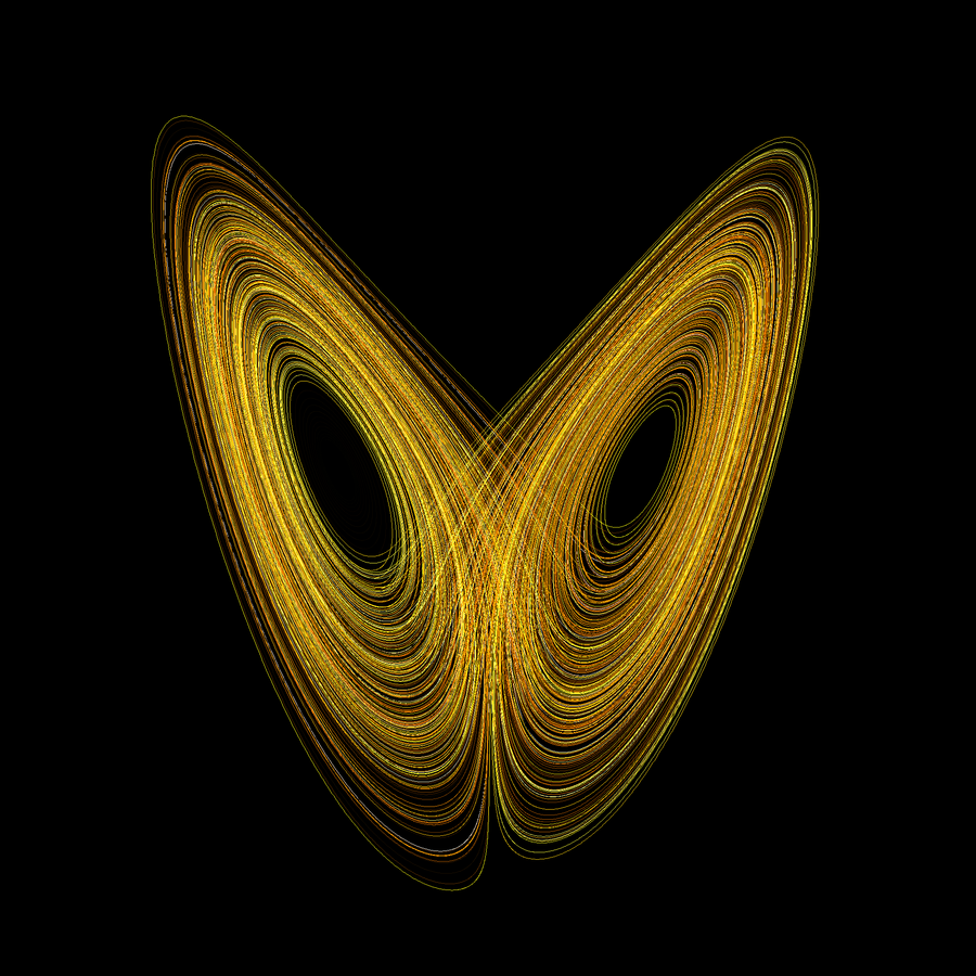
Finally the most fascinating feature are so called strange attractors. These are regions of the phase space that attract solutions, but where solutions neither converge to equilibria, nor settle into periodic orbits: instead they follow a chaotic trajectory indefinitely.