1 Introduction
The goal of Chapter 1 is to give an overview of the main themes of the course, without going into too much detail. The details will follow in subsequent chapters.
\(\text{ }\)High-level description. Differential equations are ubiquitous in mathematical modelling in physics, biology, economics and beyond. They model systems that
evolve continuously in time, and
have a “feedback mechanism” that affects how system evolves depending on the current state.
Here are some more concrete examples:
| Quantity modeled | Feedback mechanism |
|---|---|
| Motion of a physical object | Friction |
| Size of a population | Competition for resources |
| Interest rates | Market reaction |
Modeling with differential equation is however not limited to systems that match the above description. Furthermore, differential equations and their solutions are important in their own right as fundamental objects of interest in pure mathematics.
As are many of the examples and exercises of these lecture notes, this was borrowed from H. S. Bear - Differential Equations, A Concise Course.
\(\text{ }\)The meaning of Ordinary A differential equation for a function of one variable, like \(f(x)\) in ([eqn:first_eq]) which is a function only of \(x\in\mathbb{R},\) is called an Ordinary Differential Equation (ODE). In contrast a differential equation for an unknown which is a function of more than one variable (like \(f(x,y)\)), and involves partial derivatives (like \(\frac{\partial f(x,y)}{\partial x},\frac{\partial f(x,y)}{\partial y},\frac{\partial^{2}f(x,y)}{\partial x\partial y},....\)) is called a Partial Differential Equation (PDE). The expression \(\frac{\partial^{2}f(x,y)}{\partial x^{2}}+\frac{\partial^{2}f(x,y)}{\partial y^{2}}=0\) is an example of a PDE. PDEs are beyond the scope of this course, but they will be the subject of a later course.
In this course we study Ordinary Differential Equations (ODEs) and their solutions.
1.1 Deriving a differential equation in a simple physical model
This section gives an example of a derivation of a model formulated as an ODE.
\(\text{ }\)Model of object falling due to gravity Imagine an object dropped from a high tower and falling due to gravity. Let us model how its velocity evolves with time. To do so using formulas we denote the instantaneous velocity towards the ground of the object \(t\) seconds after being dropped by \(v(t).\) We assume that the object is indeed dropped and not thrown, so that the initial velocity is zero: \[v(0)=0.\tag{1.3}\] The effect of gravity is modeled by Newton’s second law of motion, which states that \[\text{force}=\text{mass}\times\text{acceleration},\tag{1.4}\] i.e. the instantaneous acceleration of an object multiplied by its mass equals the force applied to the object (at every instant of time). Acceleration is the instantaneous rate of change of velocity, i.e. \(v'(t)\) in the present setup. Let us denote the mass of the object by \(m,\) and the force exerted on the object at time \(t\) by \(f(t).\) Then Newton’s second law ([eqn:newton_2nd_law]) implies that \[v'(t)=\frac{f(t)}{m}\text{ for all }t\ge0.\tag{1.5}\] The downward force gravity exerts on an object which is much less massive than the earth close to the earths surface can be approximated by \[f_{{\rm grav}}=gm\text{ where }g=9.81.\] If we only model the force due to gravity then \(f(t)=f_{{\rm {\rm grav}}}\) for all \(t\ge0,\) so from ([eqn:newton_2nd_law_as_ODE]) we arrive at a model expressed by the equation \[v'(t)=g\text{ for all }t\ge0.\tag{1.6}\]
\(\text{ }\)Solution by integrating. To solve the model we must find the value of \(v(t)\) for all \(t\ge0.\) For the model ([eqn:grav_model]) this is a simple integration problem: by integrating both sides we find that ([eqn:grav_model]) implies \[\int_{0}^{t}v'(t)dt=\int_{0}^{t}gdt\text{ for all }t\ge0.\] By the fundamental theorem of calculus \(\int_{0}^{t}v'(t)dt=v(t)-v(0),\) and \(\int_{0}^{t}gdt=gt\) since its the integral of a constant. Using also the condition ([eq:grav_mod_init]) the solution of the model is \[v(t)=gt\text{ for all }t\ge0.\tag{1.7}\] Thus velocity increases linearly in time (this does of course not take into account that the object will eventually hit the ground, which is an effect we refrain from modeling).
\(\text{ }\)Modeling effect of air resistance. Let us include the effect of air resistance in our model. We use the (very) rough approximation that the force an object experiences due to air resistance is linear in the velocity \(v,\) i.e. \[f_{\text{air}}=-\gamma v,\] for a coefficient \(\gamma>0\) (the sign of \(f_{\text{air}}\) is opposite that of the velocity \(v,\) since air resistance acts counter to the direction of motion). In an updated model with air resistance we have \(f(t)=f_{\text{grav}}+f_{\text{air}},\) so the model we derive from Newton’s second law ([eqn:newton_2nd_law_as_ODE]) is now \[v'(t)=g-\frac{\gamma}{m}v(t)\text{ for all }t\ge0.\tag{1.8}\] This is a bona fide differential equation! The unknown function is \(v(t)\) and the equation involves both \(v(t)\) itself and its first derivative \(v'(t),\) rather than just \(v'(t)\) as in ([eqn:no_air_res_sol]).
\(\text{ }\)Difficulty of solving ([eqn:ch1_grav_model_with_air_res]) compared to ([eqn:grav_model]). The equation ([eqn:ch1_grav_model_with_air_res]) states that the rate of change of \(v(t)\) is given by the r.h.s. \(g-\frac{\gamma}{m}v(t),\) whose first term \(g\) simply represents a constant rate of increase of \(v(t),\) while the second term \(-\frac{\gamma}{m}v(t)\) depends on the current value of \(v(t)\) and is thus a feedback mechanism. Unlike the equation ([eqn:grav_model]), the equation ([eqn:ch1_grav_model_with_air_res]) does not directly allow us to compute \(v'(t)\) without already knowing \(v(t).\) Indeed if we attempt to find \(v(t)\) by integrating both sides of ([eqn:ch1_grav_model_with_air_res]), like we did to ([eqn:grav_model]) to arrive at the solution ([eqn:no_air_res_sol]) of the simpler model, we obtain \[v(t)=gt-\int_{0}^{t}\frac{\gamma}{m}v(s)ds.\] This is not very helpful, since we can’t deduce the value of the l.h.s \(v(t)\) from the r.h.s. without knowing the value of \(v(s)\) for all \(0\le s\le t.\) If we instead solve for \(v(t)\) in ([eqn:ch1_grav_model_with_air_res]) we obtain \[v(t)=\frac{m}{\gamma}(g-v'(t)),\] which suffers from the same problem: something unknown appears on both sides. The unknown function \(v(t)\) and its unknown derivative \(v'(t)\) can thus not be considered separately; we must simultaneously solve for \(v(t)\) and \(v'(t).\) This is a key feature of all differential equations.
1.2 Graphical solution of model ([eqn:ch1_grav_model_with_air_res])
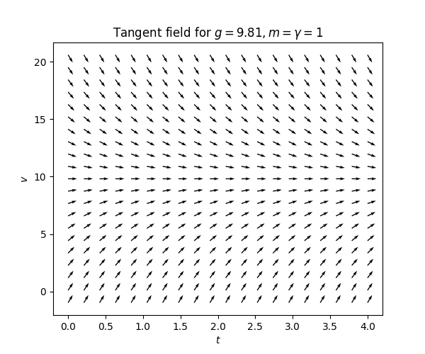
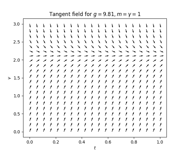
\(\text{ }\)Tangent fields Let us assume that \(m=1\) (the mass is one kg) and \(\gamma=1\) (for simplicity, this may not be a physically reasonable choice). Consider for instance \(v'(1),\) the rate of change of \(v(t)\) at time \(t=1.\) As mentioned above, the equation ([eqn:ch1_grav_model_with_air_res]) does not immediately tell us the value of \(v'(1),\) since we a priori don’t know \(v(1).\) But if we assume that e.g. \(v(1)=2,\) then ([eqn:ch1_grav_model_with_air_res]) implies that \[v'(1)=g-\frac{\gamma}{m}2=9.81-2=7.81.\] That is, if the solution \(v(t)\) satisfies \(v(1)=2,\) then the slope of the solution at \(t=1\) is \(7.81.\) This procedure can be carried out for any value of \(t\) and assumed value for \(v(t).\) We can represent all this information visually by making a plot with axes \(t\) and \(v,\) and for many different points \((t,v)\) drawing a short line segment with slope \(g-\frac{\gamma}{m}v.\) Such a plot is called a tangent field. For ([eqn:ch1_grav_model_with_air_res]) we obtain:
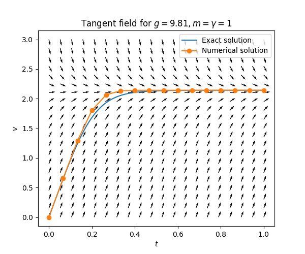
We can now pick any starting point \((t,v),\) and from there trace a curve whose slope coincides with the slope of the short lines it passes through. For instance, starting at \((t,v)=(0,0)\) we trace out the following curve:
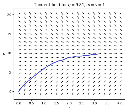
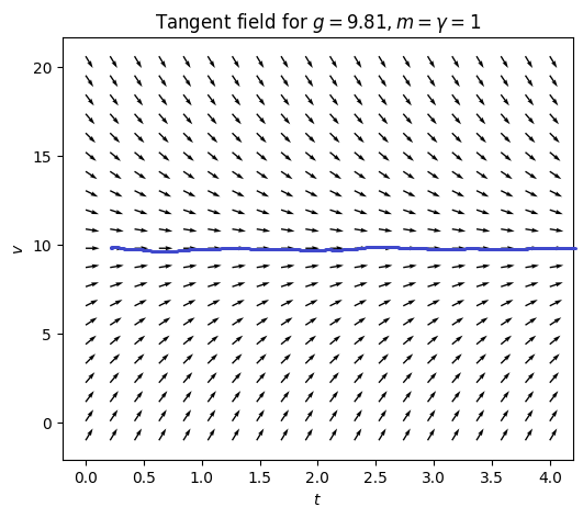
This is indeed an approximation of a solution to the differential equation ([eqn:ch1_grav_model_with_air_res])! An interesting feature of the tangent field in Figure Figure 1.1 is the arrows that point straight to the right in the middle. If one traces out a curve starting on this line, it stays on the line forever:
It should be noted that only a limited class of ODEs can be “solved” like this (essentially only first order ODEs - ODEs that involve only the first derivative without higher derivatives).
1.3 Guessing solutions
This loan-word from German is used in mathematics and means assumption or guess.
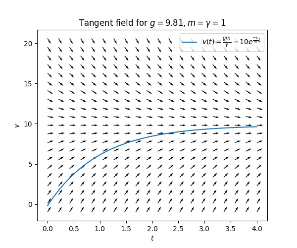
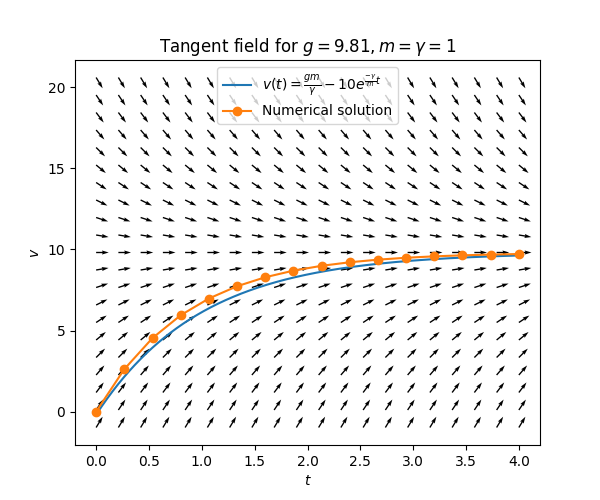
\(\text{ }\)Non-stationary solutions. Now look again at the curve traced out in Figure Figure 1.2. Does this look like the graph of some standard function? Yes, the shape is similar to that of the function \(t\to-e^{-t}\)! Motivated by this we try another ansatz: \(v(t)=a-be^{-ct}\) for some \(a,b,c\in\mathbb{R}\) to be determined. We require also \(b\ne0,c\ne0,\) since otherwise we will simply recover the stationary solution. For this ansatz we have \(v'(t)=cbe^{-ct},\) and plugging this into ([eqn:ch1_grav_model_with_air_res]) we obtain \[cbe^{-ct}=g-\frac{\gamma}{m}(a-be^{-ct}).\] If \(a,b,c\) are such that this equation holds for all \(t,\) then \(v(t)=a-be^{-ct}\) is a solution to the differential equation ([eqn:ch1_grav_model_with_air_res]). For this to happen the coefficient of the term \(e^{-ct}\) must be the same on both sides, so it must hold that \(cb=b\frac{\gamma}{m},\) implying \(c=\frac{\gamma}{m}.\) Furthermore the constant terms on both sides must coincide, so one must have \(0=g-\frac{\gamma}{m}a\) (cf. ([eq:stationary_sol])). Thus it must hold that \(a=\frac{gm}{\gamma}.\) The coefficient \(b\) can take any value. We have thus learned that \[v(t)=\frac{gm}{\gamma}-be^{-\frac{\gamma}{m}t}\] is a solution to ([eqn:ch1_grav_model_with_air_res]) for any \(b\in\mathbb{R}.\) For instance, for \(b=10\) this solution looks as follows:
Guessing the form of a solution with some “free parameters” (like \(a,b,c\) above) and then checking if any values of the parameters indeed yield a true solution is actually an important way to solve ODEs explicitly. Its somewhat fancy name is “method of undetermined coefficients”. We will use this method many times in the course.
1.4 Numerical solution
\(\text{ }\)ODE without explicit solution. It is very easy to come up with an ODE whose solutions are not given by any closed-form formula. For instance, if we make the last term of ([eqn:ch1_grav_model_with_air_res]) cubic rather than linear in \(v(t)\) we obtain the ODE \[v'(t)=g-\frac{\gamma}{m}v(t)^{3}\text{ for }t\ge0.\tag{1.13}\] The solutions of this ODE are not given by explicit formulas, except for its stationary solution. (If the last term is quadratic in \(v\) the solutions are explicit and given in terms of the hyperbolic tangent function \(\tanh\)). We can still “visually” solve ([eqn:grav_air_resist_with_third_power]) using its tangent field:
\(\text{ }\)Approximation algorithms We can also use a computer and an appropriate algorithm to compute approximations of the solutions. This simplest method is to approximate the solution by a function that is piece-wise linear on small intervals of \(t,\) where the slope at the beginning of each step (i.e. interval) is given by the slope of the tangent field at that point. Approximating a solution to equation ([eqn:grav_air_resist_with_third_power]) starting at \((t,v)=(0,0)\) with \(15\) steps yields the following curve (in orange):
To increase the accuracy of the approximation one can increase the number of steps. In fact, since there is no explicit formula for this solution the blue “exact” curve was computed in this way. Approximating the exact solution in Figure Figure 1.4 with this algorithm yields:
This simple algorithm is called the forward Euler method. We will see a modified version which applies also to ODEs of higher order (involving derivatives higher than the first). But there are ODEs for which this simple method yields very bad approximations, except with an impractically small step-size. For such ODEs more sophisticated algorithms are required. The last part of the course will deal with numerical solutions of ODEs.
1.5 Existence and uniqueness theorems
An important part of ODE theory is conditions under which solutions are guaranteed to exist, even when the equations can’t be solved explicitly. There are also conditions under which the solutions are guaranteed to be unique. For the equations discussed in Sections 1.1 - 1.4 it’s intuitively clear that for each point \((t,v)\) there is a unique solution curve passing through that point. The precise conditions for existence and uniqueness of solutions will be studied in detail later in the course.
1.6 Overview of course
In this course you will learn about
the precise definition of an Ordinary Differential Equation,
properties many different important classes of Ordinary Differential Equations,
techniques for finding explicit formulas for solutions when they exist,
theoretical guarantees for the existence and uniqueness of solutions,
numerical algorithms for approximating solutions.
2 Solutions to ODEs
In this chapter we go into the details of
what a differential equation is, and
what a solution to a differential equation is,
taking an algebraic point of view (that is, at the level of formulas).
2.1 Verifying solutions
A differential equation is a condition for an unknown function and its derivatives. Consider for instance the differential equation \[f'(t)+f(t)=0\text{ for all }t\in\mathbb{R}.\tag{2.1}\] Here the condition is “the function \(f(t)\) plus its derivative \(f'(t)\) should equal \(0\) for all \(t\)”. A solution is any function \(f\) that satisfies the condition. In this case \(f(t)=e^{-t}\) is a solution, since \[f(t)=e^{-t}\implies f'(t)=-e^{-t},\] so that if \(f(t)=e^{-t}\) then indeed \[f'(t)+f(t)=-e^{-t}+e^{-t}=0\text{ (for all }t)\checkmark.\] On the other hand, e.g. \(f(t)=t^{2}\) is not a solution to the differential equation ([eqn:ch2_first_diff_eq]), because \[f(t)=t^{2}\implies f'(t)=2t,\] so if \(f(t)=t^{2}\) then \[f'(t)+f(t)=2t+t^{2}\ne0,\] (except for \(t=0,-\frac{1}{2},\) definitely not for all \(t\in\mathbb{R}\)). A differential equation can have several, one or no solutions. E.g. \(f(t)=10e^{-t}\) is also a solution to the differential equation ([eqn:ch2_first_diff_eq]), since \[f(t)=10e^{-t}\implies f'(t)=-10e^{-t},\] so that if \(f(t)=10e^{-t}\) then indeed \[f'(t)+f(t)=-10e^{-t}+10e^{-t}=0\text{ (for all }t)\checkmark.\] In fact it is easy to see that \(f(t)=ae^{-t}\) for any fixed number \(a\) is a solution to the differential equation ([eqn:ch2_first_diff_eq]).
Another example is \[g'(x)-10g(x)=1\text{ for all }x\in\mathbb{R}.\tag{2.2}\] This equation has the solution \(g(x)=-\frac{1}{10}+e^{10x},\) since if \(g(x)=-\frac{1}{10}+e^{10x}\) then \(g'(x)=10e^{10x}\) and so \[g'(x)-10g(x)=e^{10x}-10\left(-\frac{1}{10}+e^{10x}\right)=e^{10x}+1-e^{10x}=1\text{ for all }x\in\mathbb{R}\checkmark.\]
The variable \(t\) in the equation ([eqn:ch2_first_diff_eq]) or \(a\) in ([eqn:ch2_sec_diff_eq]) is called the independent variable. It can also be represented by any other letter, such as \(s,r,u,v,a,b,c\ldots\alpha,\beta,\gamma\ldots.\) The function we are solving for is denoted by \(f\) in the equation ([eqn:ch2_first_diff_eq]) and \(g\) in ([eqn:ch2_sec_diff_eq]). It can also be represented by any other letter, e.g. \(g,h,u,v,a,b,c,\ldots,\alpha,\beta,\gamma\ldots.\). The unknown function can also be referred to as the dependent variable.
Here are some more examples of differential equations.
In the following ODE the derivative is multiplied by a non-constant term \(s\): \[sh'(s)-h(s)=0\text{ for all }s\in\mathbb{R}.\tag{2.3}\] The function \(h(s)=s\) is a solution, since if \(h(s)=s\) then \(h'(s)=1\) so \[h(s)=s\implies sh'(s)-h(s)=s\cdot1-s=0\text{ for all }s\in\mathbb{R}.\]
This ODE has a second order derivative \[u''(r)+u(r)=0\text{ for all }r\in\mathbb{R}.\tag{2.4}\] The function \(u(r)=\cos(r)\) solves it, since if \(u(r)=\cos(r)\) then \(u'(r)=-\sin(r)\) and \(u''(r)=-\cos(r)\) so \[u(r)=\cos(r)\implies u''(r)+u(r)=-\cos(r)+\cos(r)\text{ for all }r\in\mathbb{R}.\] We call ([eqn:ch2_first_diff_eq]), ([eqn:ch2_sec_diff_eq]) and ([eq:first_lin_eq_non_const_coeffs]) first order ODEs because the highest derivative that appears is the first derivative. Similarly ([eqn:ch2_sec_diff_eq]) is called a second order ODE, since the highest derivative appearing is the second. It is thus no surprise that an ODE whose highest order derivative is a \(k\)-th derivative is called a \(k\)-th order ODE. So for instance \[s'''(z)+10s'(z)-zs(z)=1.\tag{2.5}\] It is customary to order the derivatives appearing in an ODE from highest to lowest order, as in ([eqn:ch2_first_diff_eq]), ([eqn:ch2_sec_diff_eq]),([eq:first_lin_eq_non_const_coeffs]), ([eq:first_sec_order_diff_eq]), ([eq:first_third_order_eq]), but this of course not required.
The following ODE contains non-linear functions of the unknown function \(f\) and its derivatives: \[\left(f''(t)-f(t)\right)^{2}+f'(t)=0\text{ for all }t\in\mathbb{R}.\tag{2.6}\]
Use the following quiz to practice checking if a given function is a solution to an ODE or not.
2.2 Formal definition
We summarize the terminology introduced above in the following formal definition of an ODE and a solution to an ODE.
v3: added “implicit”
Note that the interval \(I\) can be finite like \((-1,1)\) or \([-1,1)\) or \([-1,1],\) or infinite like \([0,\infty)\) or all of \(\mathbb{R}.\)
For instance, ([eq:first_third_order_eq]) has this form with \(k=3\) and \[G(z,s_{3},s_{2},s_{1},s_{0})=s_{3}+10s_{1}-zs_{0}-1\] since indeed the equations \(G(z,s'''(z),s''(z),s(z),s(z))=0\) and ([eq:first_third_order_eq]) are equivalent.
Practice the definition by answering the following questions.
E.g. in the ODE ([eqn:ch2_sec_diff_eq]) the independent variable \(x\) does not appear except as an argument of \(f,\) while in the ODE ([eq:first_lin_eq_non_const_coeffs]) the independent variable appears also outside an argument of \(h.\) ODEs of the first type are called autonomous:
If \(k\ge1\) and \(G:\mathbb{R}^{k+1}\to\mathbb{R}\) and \(I\subset\mathbb{R}\) is an interval we call the expression \[G(f^{(k)}(t),f^{(k-1)}(t),\ldots,f^{'}(t),f(t))=0\quad t\in I,\tag{2.8}\] an autonomous Ordinary Differential Equation of order \(k.\) Equivalently, if the \(G\) in ([eqn:ODE_def]) does not depend on \(t,\) then ([eqn:ODE_def]) is an autonomous ODE.
The solutions of an autonomous evolve the same way when the solution takes the same value, regardless of the value of the independent variable.
2.3 Method of undetermined coefficients
Consider the second order equation \[f''(x)+4f(x)=0\quad\quad x\in\mathbb{R}.\] If we are told that this equation has a solution of the form \(f(x)=a\cos(bx)\) (for \(a\ne0\)), we can easily verify the claim and if its true find the corresponding solutions. We simply note that if \(f(x)=a\cos(bx)\) then \(f'(x)=-ab\sin(bx)\) and \(f''(x)=-ab^{2}\cos(bx),\) so then \[f''(x)+f(x)=-ab^{2}\cos(bx)+a4\cos(bx).\] For \(f(x)=a\cos(bx)\) to be a solution this must be identically zero, that is zero for all \(x\in\mathbb{R}.\) This can only happen if the \(\cos\) terms cancel, so for an \(f(x)\) of this form to be a solution it must hold that \(ab^{2}=4a,\) which turn is equivalent to \(b=\pm2\) (since we assumed \(a\ne0\)). This implies that \(a\cos(2x)\) and \(a\cos(-2x)\) are solutions. By the identity \(\cos(x)=\cos(-x)\) they are in fact the same solution. If we aren’t completely sure that we didn’t make a mistake we can easily double check the result by simply plugging \(f(x)=a\cos(2x)\) into the equation and verify the solution like we did in Section 2.1. In this case \(f(x)=a\cos(2x)\implies f'(x)=2a\cos(2x)\implies f''(x)=4a\cos(2x)\) so indeed \[f''(x)+f'(x)=4a\cos(2x)-4a\cos(2x)=0.\] Guessing the form of a solution and then solving scalar equations to check if there is indeed a solution of that form like we did above is sometimes called the “method of undetermined coefficients”. Despite its simplicity it is in fact an important technique for explicitly solving ODEs. Practice with the following quiz.
2.4 Alternative notation
In this section you will learn some common alternative ways to write ODEs.
Firstly, one often drops the dependent variable from the argument of the function for compactness, writing instead of e.g. ([eqn:alg_non_lin_eq]) \[\left(f''-f\right)^{2}+f'=0\text{ for all }t\in\mathbb{R}.\tag{2.10}\] An alternative way to write the derivatives is using Newton’s notation: \(\dot{f}\) for the first derivative, \(\ddot{f}\) for the second, \(\dddot{f}\) for the third (if one wants to indicate the independent variable: \(\dot{f}(t),\ddot{f}(t),\dddot{f}(t)\)) . When writing derivatives like this or like in ([eqn:alg_non_lin_eq_wo_indep_var]) one usually writes fourth and higher derivatives as \(f^{(4)},f^{(5)},\ldots.\) One can also write \(f^{(0)},f^{(1)},f^{(2)},f^{(3)}\) for the function and its first, second and third derivatives respectively. Finally one can also use Leibniz’s notation for the derivatives, denoting the first derivative by \(\frac{df}{dx}\) and the \(k\)-th derivative by \(\frac{d^{k}f}{dx^{k}}.\) Thus ([eqn:alg_non_lin_eq_wo_indep_var]) is the same as \[\left(\ddot{f}-f\right)^{2}+\dot{f}=0\text{ for all }t\in\mathbb{R}\quad\quad\text{ or }\quad\quad\left(\frac{d^{2}f}{dx^{2}}-f\right)^{2}+\frac{df}{dx}=0\text{ for all }t\in\mathbb{R}.\] Practice these notations with this quiz:
\[g''-g'+\cos(x)g=0.\]
Yes, the name of the function, the name of independent variable and the name the notaton for the derivative is different, but the equatoin represented is exactly the same: \(f \iff u,\) \(x \iff s,\) \(f''' \iff \dddot{u}.\)
No: the first equaton involves a second derivative of the unkown function \(\alpha,\) while the second does not involve the second derivative \(t''(y).\)
3 First order equations
If \(k\ge1\) and \({G:\mathbb{R}^{k+2}\to\mathbb{R}}\) and \(I\subset\mathbb{R}\) is an interval we call the expression \[G(t,f^{(k)}(t),f^{(k-1)}(t),\ldots,f^{'}(t),f(t))=0\quad t\in I,\tag{2.7}\] an Ordinary Differential Equation of order \(k.\) We call any \(k\)-times differential function \(h:I\to\mathbb{R}\) such that \[G(t,h^{(k)}(t),h^{(k-1)}(t),\ldots,h^{'}(t),h(t))=0\quad\forall t\in I,\] solution to the ODE ([eqn:ODE_def]) on the interval \(I.\)
3.1 Tangent fields
In this section you will practice working with tangent fields.
In Section 1.2 we saw that a tangent field can be used to visualize solutions of a first order ODE. Other common names for these plots include slope field or direction field. Recall that a tangent field is a plot where at many possible values of the dependent and independent variables a short line segment or arrow indicates the slope of a solution that passes through that point.
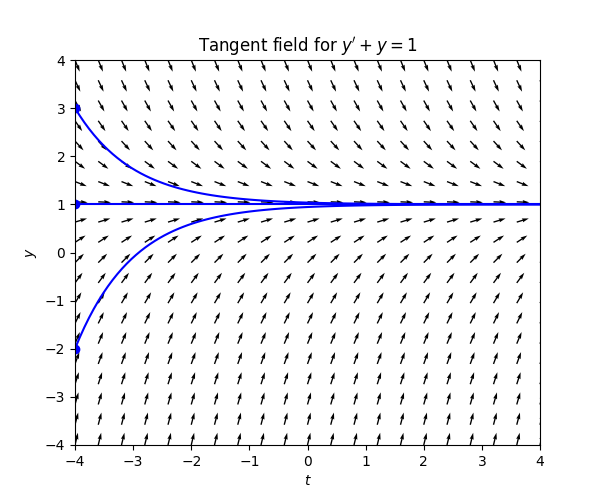
Consider the ODE \[y'+y=1.\tag{3.2}\] To draw the tangent field it is more convenient to write this as \[y'=1-y.\] From this we see that \[\text{the tangent at point }(t,y)\text{ has slope }1-y.\] Thus for instance if \(y=0\) the slope is \(1,\) i.e. the tangent should point up \(45\) degrees, like the slope of the function \(f(x)=x.\) If \(y=2\) the slope is \(-1,\) so the tangent should point down \(45\) degrees, like the slope of the function \(f(x)=-x.\) For \(y>1\) the slope is negative and so the tangents point down. For \(y<1\) the slope is positive and the tangents point up. For \(y=1\) the slopes are zero. The slopes become become steeper as \(y\) moves away from \(1.\) This is the resulting tangent field:
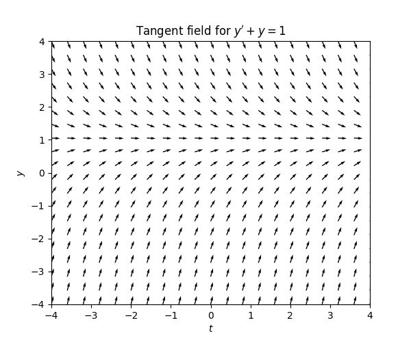
If \(y>1\) the slopes “force” the solution down to \(1,\) and if \(y<1\) the slopes “force” the solutions up to \(1.\) If \(y=1\) constantly then the slopes are zero: this is a stationary solutions. Since the slope is less steep closer to \(y=1,\) the solutions “slow down” with time: the rate of approaching \(y=1\) decreases with time. Here is the tangent field with some solution curves:
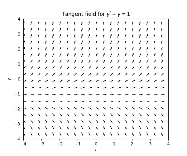
Consider the ODE \[y'-y=1.\tag{3.3}\] Writing this as \[y'=1+y,\] we see that in the tangent field \[\text{the tangent at point }(t,y)\text{ has slope }1+y.\] If \(y=0\) the slope is \(1\) and if \(y=-2\) the slope is \(-1.\) For \(y>-1\) the slope is positive and so the tangents point up. For \(y>-1\) the slope is negative and the tangents point down. For \(y=-1\) the slopes are zero. The slopes become become steeper as \(y\) moves away from \(-1.\) This is the resulting tangent field:
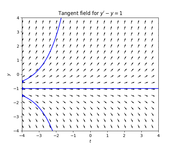
If \(y>-1\) the slopes “force” the solution upwards at an increasing rate, and if \(y<-1\) the slopes “force” the solutions downwards at an increasing rate. For \(y=-1\) the slopes are zero so this is a stationary solution.. Here is the tangent field with some solution curves:
Consider the ODE \[y'-y=1.\tag{3.3}\] Writing this as \[y'=1+y,\] we see that in the tangent field \[\text{the tangent at point }(t,y)\text{ has slope }1+y.\] If \(y=0\) the slope is \(1\) and if \(y=-2\) the slope is \(-1.\) For \(y>-1\) the slope is positive and so the tangents point up. For \(y>-1\) the slope is negative and the tangents point down. For \(y=-1\) the slopes are zero. The slopes become become steeper as \(y\) moves away from \(-1.\) This is the resulting tangent field:
If \(y>-1\) the slopes “force” the solution upwards at an increasing rate, and if \(y<-1\) the slopes “force” the solutions downwards at an increasing rate. For \(y=-1\) the slopes are zero so this is a stationary solution.. Here is the tangent field with some solution curves:
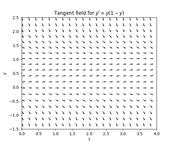
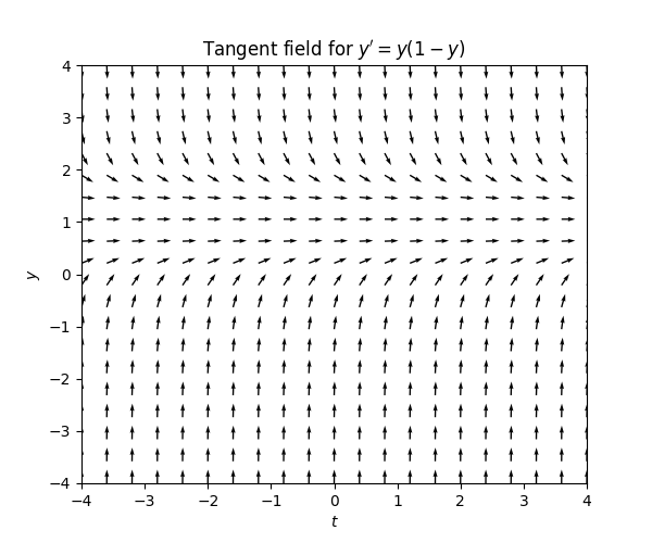
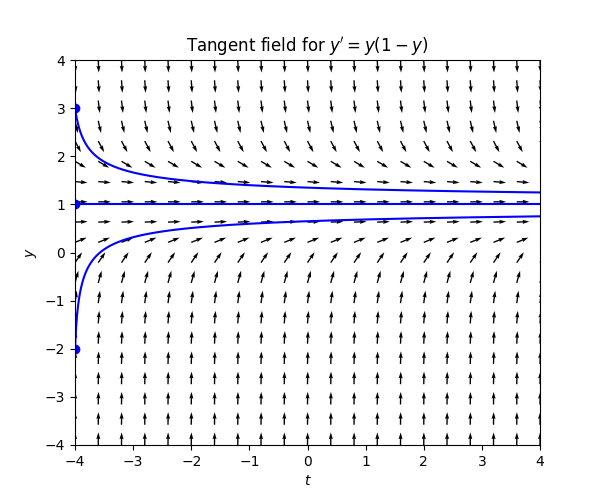
Consider the ODE \[y'=y(1-y).\tag{3.4}\] The r.h.s. is zero if \(y=0\) or \(y=1,\) so there the slopes are zero. For \(y\in(0,1)\) the r.h.s. and the slopes are positive, and for \(y>1\) and \(y<0\) the the r.h.s. and the slopes are negative. The magnitude of the slopes decreases as you get closer to \(0,1.\) This is the resulting tangent field:
Between \(y=0\) and \(y=1\) the slopes force the solution upwards to \(y=1,\) which is a stationary solution, and for \(y>1\) the slopes force the solution downwards to \(y=1.\) For \(y<0\) the slopes for the solution down to \(-\infty.\) Here is the tangent field with some solution curves:
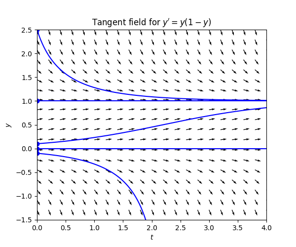
The ODE ([eq:tangent_field_ex_3_eq]) is called the logistic equation. It can serve as a simple model for the size of a biological population. A positive value of \(y(t)\) close to zero is interpreted as a small population, and \(y(t)=1\) is interpreted as the size of population that saturates the environment so that it cannot grow any further. The population grows fast for \(y(t)\) close to \(0,\) due to absence of competition for resources, and as the population gets closer to \(y=1\) the rate of growth of the population slows. The solutions outside the interval \([0,1]\) are not meaningful from the point of view of this model.
Consider the ODE \[y'=y+t.\tag{3.5}\] The slopes are negative for \(y<-t\) and positive for \(y>-t.\) For \(y=-t\) the slope is zero. This is the resulting tangent field:
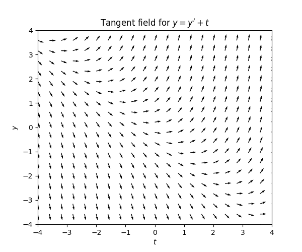
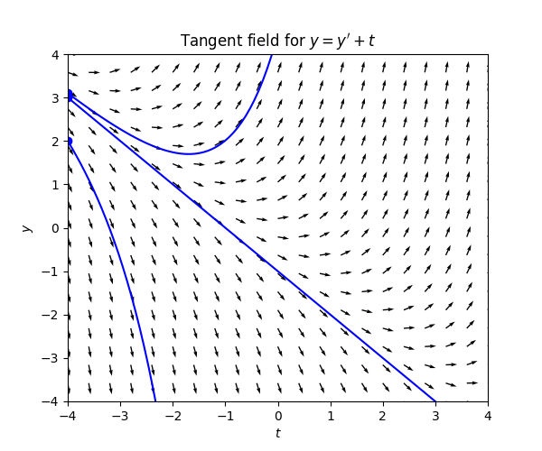
There is no stationary solution, but inspecting the tangent field there appears to be a linear solution. We can easily check if this is indeed the case as we did in Section 2.3: We make the ansatz \(y=at+b\) for \(a,b\in\mathbb{R}\) and note that then \(y'=a,\) so this linear function is a solution provided \[a=at+b+t=0\text{ for all }t\in\mathbb{R}.\tag{3.6}\] We see that if \(a=-1\) and \(b=-1\) then indeed ([eqn:tangent_lin_sol]) holds, so \(y=-t-1\) is a solution.
From the tangent field one sees that if \(y\) is below the line \(t\to-t-1\) then it is “forced” downwards away from the line, and if t is above this line it is “force” upwards away from the line. The solution \(y(t)=-t-1\) is “unstable”.
Consider the ODE \[y'+y=1.\tag{3.2}\] To draw the tangent field it is more convenient to write this as \[y'=1-y.\] From this we see that \[\text{the tangent at point }(t,y)\text{ has slope }1-y.\] Thus for instance if \(y=0\) the slope is \(1,\) i.e. the tangent should point up \(45\) degrees, like the slope of the function \(f(x)=x.\) If \(y=2\) the slope is \(-1,\) so the tangent should point down \(45\) degrees, like the slope of the function \(f(x)=-x.\) For \(y>1\) the slope is negative and so the tangents point down. For \(y<1\) the slope is positive and the tangents point up. For \(y=1\) the slopes are zero. The slopes become become steeper as \(y\) moves away from \(1.\) This is the resulting tangent field:
If \(y>1\) the slopes “force” the solution down to \(1,\) and if \(y<1\) the slopes “force” the solutions up to \(1.\) If \(y=1\) constantly then the slopes are zero: this is a stationary solutions. Since the slope is less steep closer to \(y=1,\) the solutions “slow down” with time: the rate of approaching \(y=1\) decreases with time. Here is the tangent field with some solution curves:
Consider the ODE \[y'-y=1.\tag{3.3}\] Writing this as \[y'=1+y,\] we see that in the tangent field \[\text{the tangent at point }(t,y)\text{ has slope }1+y.\] If \(y=0\) the slope is \(1\) and if \(y=-2\) the slope is \(-1.\) For \(y>-1\) the slope is positive and so the tangents point up. For \(y>-1\) the slope is negative and the tangents point down. For \(y=-1\) the slopes are zero. The slopes become become steeper as \(y\) moves away from \(-1.\) This is the resulting tangent field:
If \(y>-1\) the slopes “force” the solution upwards at an increasing rate, and if \(y<-1\) the slopes “force” the solutions downwards at an increasing rate. For \(y=-1\) the slopes are zero so this is a stationary solution.. Here is the tangent field with some solution curves:
Consider the ODE \[y'=y(1-y).\tag{3.4}\] The r.h.s. is zero if \(y=0\) or \(y=1,\) so there the slopes are zero. For \(y\in(0,1)\) the r.h.s. and the slopes are positive, and for \(y>1\) and \(y<0\) the the r.h.s. and the slopes are negative. The magnitude of the slopes decreases as you get closer to \(0,1.\) This is the resulting tangent field:
Between \(y=0\) and \(y=1\) the slopes force the solution upwards to \(y=1,\) which is a stationary solution, and for \(y>1\) the slopes force the solution downwards to \(y=1.\) For \(y<0\) the slopes for the solution down to \(-\infty.\) Here is the tangent field with some solution curves:
Consider the ODE \[y'=y+t.\tag{3.5}\] The slopes are negative for \(y<-t\) and positive for \(y>-t.\) For \(y=-t\) the slope is zero. This is the resulting tangent field:
There is no stationary solution, but inspecting the tangent field there appears to be a linear solution. We can easily check if this is indeed the case as we did in Section 2.3: We make the ansatz \(y=at+b\) for \(a,b\in\mathbb{R}\) and note that then \(y'=a,\) so this linear function is a solution provided \[a=at+b+t=0\text{ for all }t\in\mathbb{R}.\tag{3.6}\] We see that if \(a=-1\) and \(b=-1\) then indeed ([eqn:tangent_lin_sol]) holds, so \(y=-t-1\) is a solution.
From the tangent field one sees that if \(y\) is below the line \(t\to-t-1\) then it is “forced” downwards away from the line, and if t is above this line it is “force” upwards away from the line. The solution \(y(t)=-t-1\) is “unstable”.
If \(k\ge1\) and \(G:\mathbb{R}^{k+1}\to\mathbb{R}\) and \(I\subset\mathbb{R}\) is an interval we call the expression \[G(f^{(k)}(t),f^{(k-1)}(t),\ldots,f^{'}(t),f(t))=0\quad t\in I,\tag{2.8}\] an autonomous Ordinary Differential Equation of order \(k.\) Equivalently, if the \(G\) in ([eqn:ODE_def]) does not depend on \(t,\) then ([eqn:ODE_def]) is an autonomous ODE.
The autonomous equations ([eq:tangent_field_ex_1_eq]), ([eq:tangent_field_ex_2_eq]), ([eq:tangent_field_ex_3_eq]) are of the form \[y'=G(y),\tag{3.7}\] for \(G(y)=y,G(y)=-y,G(y)=y(1-y)\) respectively. Note that for such an ODE the stationary solutions are precisely given by \(c\in\mathbb{R}\) for which \(G(c)=0\) - indeed if \(y(t)=c\) for such a \(c\) then \(y'=0\) and \(G(y(t))=G(c)=0,\) so ([eq:ch3_tf_first_order_aut_explicit]) is satisfied.
Consider the ODE \[y'+y=1.\tag{3.2}\] To draw the tangent field it is more convenient to write this as \[y'=1-y.\] From this we see that \[\text{the tangent at point }(t,y)\text{ has slope }1-y.\] Thus for instance if \(y=0\) the slope is \(1,\) i.e. the tangent should point up \(45\) degrees, like the slope of the function \(f(x)=x.\) If \(y=2\) the slope is \(-1,\) so the tangent should point down \(45\) degrees, like the slope of the function \(f(x)=-x.\) For \(y>1\) the slope is negative and so the tangents point down. For \(y<1\) the slope is positive and the tangents point up. For \(y=1\) the slopes are zero. The slopes become become steeper as \(y\) moves away from \(1.\) This is the resulting tangent field:
If \(y>1\) the slopes “force” the solution down to \(1,\) and if \(y<1\) the slopes “force” the solutions up to \(1.\) If \(y=1\) constantly then the slopes are zero: this is a stationary solutions. Since the slope is less steep closer to \(y=1,\) the solutions “slow down” with time: the rate of approaching \(y=1\) decreases with time. Here is the tangent field with some solution curves:
Comparing the tangent field with solutions in Figure Figure 3.2 and in this case we see the effect of the difference between the steepness of the slopes: for \(y>2\) or \(y<0,\) where \(\left|y-1\right|>1,\) the solutions here “move faster” than those of in Figure Figure 3.2. If \(y\in(0,2),\) where \(\left|y-1\right|<1\) the solutions “move slower” than those in Figure Figure 3.2.
Note that a tangent field can only be drawn for a first order equation, since only then is \(y'\) a function of just \(y\) and \(t.\)
While a second order equation can be written as \(y''=G(t,y'),\) to make a plot that represents all the information about the state of the system would require a 3D plot, since there are three variables \(y'',t,y'.\) For an autonomous second order equation the \(t\) variable goes away and one could represent the system by a 2D plot again - we will probably see such phase plane plots later. But for order three and higher even autonomous equations can not be represented in a 2D plot without loss of information.
Here is quiz on tangent fields. You do not need to mathematically prove the statements here - in particular you can extrapolate the behavior of the tangents to the whole plane using.