5 Higher order linear autonomous equations
In this chapter we study \(k\)-th order linear autonomous equations of the form \[y^{(k)}(t)+\sum_{l=0}^{k-1}a_{l}y^{(l)}(t)=b,\quad\quad t\in I,\tag{5.1}\] for \(k\ge1\) and constants \(a_{l},b.\) These admit an explicit closed form solution for any value of the constants, which is hard to come by for more general higher order ODEs. Later we will study the non-autonomous case, where the coefficients \(a_{l},b\) can be functions of the independent variable \(t.\)
If \(I\) is a non-empty interval, \(k\ge1\) and \(a_{0},\ldots,a_{k-1},b\in\mathbb{R}\) we call the ODE ([eq:ch5_higher_order_lin_aut]) a \(k\)-th order linear autonomous ODE, or equivalently a \(k\)-th order linear ODE with constant coefficients.
We call any equation of the form \[\dot{y}(t)=ay(t)+b,\quad\quad t\in I,\tag{3.10}\] for \(a,b\in\mathbb{R}\) and any interval \(I\subset\mathbb{R}\) a first order linear autonomous ODE.
b) As in the first order linear autonomous case, the solutions to the ODE ([eq:ch5_higher_order_lin_aut]) are well-defined on all of \(\mathbb{R},\) so in principle we could just set \(I=\mathbb{R},\) but for consistency we keep \(I\) as a general interval.
5.1 Second order
If \(I\) is a non-empty interval, \(k\ge1\) and \(a_{0},\ldots,a_{k-1},b\in\mathbb{R}\) we call the ODE ([eq:ch5_higher_order_lin_aut]) a \(k\)-th order linear autonomous ODE, or equivalently a \(k\)-th order linear ODE with constant coefficients.
The ODE \[y''+y'-2y=-3,\quad\quad t\in\mathbb{R},\tag{5.2}\] is a second order linear autonomous equation.
The general form is \[y''+a_{1}y'+a_{0}y=b,\quad\quad\quad t\in I,\tag{5.3}\] for \(a_{1},a_{0},b\in\mathbb{R}.\)
\(\text{ }\) Stationary solution. It is easy to see that ODEs of this form always have a stationary solution. Starting with the example ([eq:ch5_so_lin_aut_first_example]), if we make the ansatz \(y(t)=c,t\in\mathbb{R},\) and note that then \(y''(t)=y'(t)=0\) we obtain the equation \[-2c=-3,\] which has the unique solution \(c=\frac{3}{2}.\) Thus \(y(t)=\frac{3}{2}\) is the unique stationary solution of ([eq:ch5_so_lin_aut_first_example]). For the general ODE ([eq:ch5_so_lin_aut_gen]) the computation is the same: the ansatz \(y(t)=c\) yields \(y''=y'=0\) and so ([eq:ch5_so_lin_aut_gen]) reduces to \[a_{0}c=b,\] with unique solution \(c=\frac{b}{a_{0}},\) so that \(y(t)=\frac{b}{a_{0}}\) is the unique stationary solution (cf. the stationary solution in the first order case ([eq:ch3_fo_lin_aut_stationary]); the difference in the sign is because the standard form we us here reduces to \(y'+a_{0}y=b\) for \(k=1,\) in contrast to \(y'=ay+b\) used in Chapter 3). Below we will consider the case \(a_{0}=0.\)
\(\text{ }\) Homogeneous equation. Like we did for first order equations, for any solution \(y\) we can subtract the stationary solution to obtain a solution of a somewhat simpler equation.
The ODE \[y''+y'-2y=-3,\quad\quad t\in\mathbb{R},\tag{5.2}\] is a second order linear autonomous equation.
In the general case we set \(x(t)=y(t)-\frac{b}{a_{0}}\) to obtain that \(y\) is a solution of ([eq:ch5_so_lin_aut_gen]) iff \(x\) is a solution of \[x''+a_{1}x'+a_{0}x=0.\tag{5.6}\] The unique stationary solution of equations ([eq:ch5_so_lin_aut_first_example_recent]) and ([eq:ch5_so_lin_aut_gen_homo]) is \(x(t)=0.\)
Equations like ([eq:ch5_so_lin_aut_first_example_recent]) and ([eq:ch5_so_lin_aut_gen_homo]), of the form ([eq:ch5_so_lin_aut_gen]) with \(b=0,\) are called a homogeneous equation. They will play an important role in the theory here and later also in the theory of higher-order non-autonomous linear ODEs.
Any ODE of the form \[y''+a_{1}y'+a_{0}y=0,\quad\quad t\in I,\tag{5.7}\] is called a \(2\)nd order homogeneous linear autonomous equation, or equivalently a 2nd order homogeneous linear ODE with constant coefficients.
An important property of homogeneous equations is that any linear combination of solutions is again a solution. This is easy to see: if \(y_{1}\) satisfies ([eq:ch5_so_lin_aut_homo_def]) then letting \(y_{2}(t)=\alpha y_{1}(t)\,\forall t\) for a constant \(\alpha\in\mathbb{R},\) then \(y_{2}'=\alpha y_{1}'\) and \(y_{2}''=\alpha y_{1}''\) so \[y_{2}''+a_{1}y_{2}''+a_{0}y_{2}=\alpha\left(y_{1}''+a_{1}y_{1}'+a_{0}y\right)=\alpha\cdot0=0,\tag{5.8}\] so \(y_{2}\) also satisfies ([eq:ch5_so_lin_aut_homo_def]). If \(y_{1},y_{2}\) satisfy ([eq:ch5_so_lin_aut_homo_def]) and \(y_{3}(t)=y_{1}(y)+y_{2}(t)\,\forall t\) then since \(y_{3}'=y_{1}'+y_{2}'\) and \(y_{3}''=y_{1}''+y_{2}''\) it holds that \[\begin{array}{ccl} y_{3}''+a_{1}y_{3}'+a_{0}y_{3} & = & \left(y_{1}''+y_{2}''\right)+a_{1}(y_{1}'+y_{2}')+a_{0}(y_{1}+y_{2})\\ & = & \left(y_{1}''+a_{1}y_{1}'+a_{0}y_{1}\right)+\left(y_{2}''+a_{1}y_{2}'+a_{0}y_{2}\right)\\ & = & 0+0=0, \end{array}\tag{5.9}\] for all \(t,\) so \(y_{3}\) also satisfies ([eq:ch5_so_lin_aut_homo_def]). Note that these computations work out only because 1) taking the derivative is a linear operation, 2) the l.h.s. of the ODE ([eq:ch5_so_lin_aut_homo_def]) is linear in the derivatives and 3) the r.h.s. of ([eq:ch5_so_lin_aut_homo_def]) is zero. Points 1) and 2) still apply in the non-homogeneous case ([eq:ch5_so_lin_aut_gen]), \(b\ne0,\) but 3) does not: starting with a solution to ([eq:ch5_so_lin_aut_gen]) in ([eq:ch5_so_lin_homo_mult_lin]) and ([eq:ch5_so_lin_homo_sum_lin]) would give a r.h.s. different from the original equation - namely \(\alpha b\) and \(b+b=2b\) respectively. We already mentioned this linear property in the context of first order linear equations in Section 3.5. As we will see indeed any homogeneous linear equation of any order - autonomous or not - has it.
The next lemma encapsulates this linearity (c) and b)) and the other important properties discussed above.
Let \(a_{0},a_{1},b\in\mathbb{R}\) and \(I\) be a non-empty interval.
a) Assume \(a_{0}\ne0.\) Then a a function \(y\) is a solution to ([eq:ch5_so_lin_aut_gen]) iff \(x=y-\frac{b}{a_{0}}\) is a solution to ([eq:ch5_so_lin_aut_homo_def]).
b) \(y(t)=0\) is a solution to ([eq:ch5_so_lin_aut_homo_def]).
c) If \(y\) is a solution to ([eq:ch5_so_lin_aut_homo_def]) then \(\alpha y\) is also a solution for any \(\alpha\in\mathbb{R}.\)
d) If \(y_{1}\) and \(y_{2}\) are solutions to ([eq:ch5_so_lin_aut_homo_def]) then \(y_{1}+y_{2}\) is also a solution to ([eq:ch5_so_lin_aut_homo_def]).
Proof. Exercise (all arguments are included in the text above).
1. Point d) is called the superposition principle.
2. Let \(\mathcal{Y}\) be the set of solutions of ([eq:ch5_so_lin_aut_homo_def]). The linearity proved by points c) d) imply that \(\mathcal{Y}\) is a vector space over \(\mathbb{R}.\)
\(\text{ }\) Exponential ansatz. In Section 3.2 we saw that first order autonomous linear equations have solutions of the form \(e^{ct}\) for a \(c\in\mathbb{R}\) depending on the coefficients of the equation. Let’s see if these second order ODEs also have such solutions.
The ODE \[y''+y'-2y=-3,\quad\quad t\in\mathbb{R},\tag{5.2}\] is a second order linear autonomous equation.
(Continuation of Example 5.3) For ([eq:ch5_so_lin_aut_first_example]) we set \(x(t)=y(t)-\frac{3}{2}\) and note that if \(y\) is a solution of ([eq:ch5_so_lin_aut_first_example]) then \[x''+x'-2x=y''+y'-2\left(y-\frac{3}{2}\right)=y''+y'-2y+3=0,\] so \(x\) is a solution of \[x''+x'-2x=0.\tag{5.5}\] In fact \(y\) is solution of ([eq:ch5_so_lin_aut_first_example]) iff \(x\) is a solution of ([eq:ch5_so_lin_aut_first_example_recent]).
Let \(a_{0},a_{1},b\in\mathbb{R}\) and \(I\) be a non-empty interval.
a) Assume \(a_{0}\ne0.\) Then a a function \(y\) is a solution to ([eq:ch5_so_lin_aut_gen]) iff \(x=y-\frac{b}{a_{0}}\) is a solution to ([eq:ch5_so_lin_aut_homo_def]).
b) \(y(t)=0\) is a solution to ([eq:ch5_so_lin_aut_homo_def]).
c) If \(y\) is a solution to ([eq:ch5_so_lin_aut_homo_def]) then \(\alpha y\) is also a solution for any \(\alpha\in\mathbb{R}.\)
d) If \(y_{1}\) and \(y_{2}\) are solutions to ([eq:ch5_so_lin_aut_homo_def]) then \(y_{1}+y_{2}\) is also a solution to ([eq:ch5_so_lin_aut_homo_def]).
\(\text{ }\) Characteristic equation. The equation ([eq:ch5_so_lin_aut_homo_examp_exp_char_eq]) is called the characteristic equation of the ODE. For the general non-homogeneous ([eq:ch5_so_lin_aut_first_example]) and homogeneous ([eq:ch5_so_lin_aut_gen_homo]) ODEs the characteristic function is \[r^{2}+a_{1}r+a_{0}=0,\tag{5.15}\] (so it does not depend on \(b\) on the r.h.s. of ([eq:ch5_so_lin_aut_first_example])). The l.h.s. of ([eq:ch5_so_lin_aut_char_eq_gen]) is called the characteristic polynomial, which for second order equations is always a quadratic polynomial. If this has real solutions \(r_{1},r_{2}\) then \(x(t)=e^{r_{1}t},x(t)=e^{r_{2}t}\) and linear combinations \(x(t)=\alpha_{1}e^{r_{1}t}+\alpha_{2}e^{r_{2}t}\) are all solutions of the homogeneous ODE ([eq:ch5_so_lin_aut_gen_homo]). If \(a_{0}\ne0\) then \(y(t)=\alpha_{1}e^{r_{1}t}+\alpha_{2}e^{r_{2}t}-\frac{b}{a_{0}}\) are solutions of the non-homogeneous ODE ([eq:ch5_so_lin_aut_gen_homo]). Below we will consider the situation where the characteristic equation ([eq:ch5_so_lin_aut_char_eq_gen]) has no real roots (like for instance \(r^{2}+1=0\) with complex roots \(r=\pm i\)).
\(\text{ }\) IVPs for second order ODEs. Now let us study IVPs when the characteristic equation has two distinct real roots.
The ODE \[y''+y'-2y=-3,\quad\quad t\in\mathbb{R},\tag{5.2}\] is a second order linear autonomous equation.
(Continuation of Example 5.3) For ([eq:ch5_so_lin_aut_first_example]) we set \(x(t)=y(t)-\frac{3}{2}\) and note that if \(y\) is a solution of ([eq:ch5_so_lin_aut_first_example]) then \[x''+x'-2x=y''+y'-2\left(y-\frac{3}{2}\right)=y''+y'-2y+3=0,\] so \(x\) is a solution of \[x''+x'-2x=0.\tag{5.5}\] In fact \(y\) is solution of ([eq:ch5_so_lin_aut_first_example]) iff \(x\) is a solution of ([eq:ch5_so_lin_aut_first_example_recent]).
(Continuation of Example 5.3 and Example 5.4) We make the ansatz \(x(t)=e^{rt}\) for some \(r\in\mathbb{R}\) in ([eq:ch5_so_lin_aut_first_example_recent]), i.e. in the ODE \[x''+x'-2x=0.\tag{5.11}\] With this ansatz \(x'(t)=re^{r}\) and \(x''(t)=r^{2}e^{rt},\) so the equation reduces to \[r^{2}e^{rt}+re^{rt}-2e^{rt}=0.\tag{5.12}\] The term \(e^{rt}\) (which is always non-zero) can be factored out to obtain \[r^{2}+r-2=0.\tag{5.13}\] This is quadratic equation for \(r\) which can be factored as \[(r-1)(r+2)=0,\tag{5.14}\] and thus has roots \(r_{1}=1,r_{2}=-2.\) Therefore if \(x(t)=e^{rt}\) with \(r=r_{1}\) or \(r=r_{2}\) then ([eq:ch5_so_lin_aut_homo_examp_exp_char_eq_factored]), ([eq:ch5_so_lin_aut_homo_examp_exp_char_eq]), ([eq:ch5_so_lin_aut_homo_examp_exp_ansatz_ODE_plugged_in]) and ([eq:ch5_so_lin_aut_homo_examp_exp_ansatz_ODE]) are all satisfied, so \(x(t)\) is a solution. Also \(x(t)=e^{rt}\) satisfy these identically for all \(t\) only if \(r=r_{1}\) or \(r=r_{2},\) so there are no other solutions of this form. By Lemma 5.6 c) d) we also see that for any \(\alpha_{1},\alpha_{2}\in\mathbb{R}\) \[\alpha_{1}e^{t}+\alpha_{2}e^{-2t},\] is a solution to ([eq:ch5_so_lin_aut_homo_examp_exp_ansatz_ODE]).
By Lemma 5.6 a) \[y(t)=\alpha_{1}e^{t}+\alpha_{2}e^{-2t}+\frac{3}{2},\] for \(r=r_{1}\) or \(r=r_{2}\) and any \(\alpha_{1},\alpha_{2}\in\mathbb{R}\) are solutions to the associated non-homogeneous ODE ([eq:ch5_so_lin_aut_first_example]).
(Complete solution of first order autonomous ODEs with \(a\ne0\)). Assume \(a,b\in\mathbb{R},a\ne0\) and \(I\subset\mathbb{R}\) an interval. Then a function \(y(t)\) is a solution of the ODE \[\dot{y}(t)=ay(t)+b,\quad\quad t\in I,\tag{3.23}\] iff \[y(t)=\alpha e^{at}-\frac{b}{a}\quad\forall t\in I,\text{ for some }\alpha\in\mathbb{R}.\tag{3.24}\]
The ODE \[y''+y'-2y=-3,\quad\quad t\in\mathbb{R},\tag{5.2}\] is a second order linear autonomous equation.
(Continuation of Example 5.3) For ([eq:ch5_so_lin_aut_first_example]) we set \(x(t)=y(t)-\frac{3}{2}\) and note that if \(y\) is a solution of ([eq:ch5_so_lin_aut_first_example]) then \[x''+x'-2x=y''+y'-2\left(y-\frac{3}{2}\right)=y''+y'-2y+3=0,\] so \(x\) is a solution of \[x''+x'-2x=0.\tag{5.5}\] In fact \(y\) is solution of ([eq:ch5_so_lin_aut_first_example]) iff \(x\) is a solution of ([eq:ch5_so_lin_aut_first_example_recent]).
(Continuation of Example 5.3 and Example 5.4) We make the ansatz \(x(t)=e^{rt}\) for some \(r\in\mathbb{R}\) in ([eq:ch5_so_lin_aut_first_example_recent]), i.e. in the ODE \[x''+x'-2x=0.\tag{5.11}\] With this ansatz \(x'(t)=re^{r}\) and \(x''(t)=r^{2}e^{rt},\) so the equation reduces to \[r^{2}e^{rt}+re^{rt}-2e^{rt}=0.\tag{5.12}\] The term \(e^{rt}\) (which is always non-zero) can be factored out to obtain \[r^{2}+r-2=0.\tag{5.13}\] This is quadratic equation for \(r\) which can be factored as \[(r-1)(r+2)=0,\tag{5.14}\] and thus has roots \(r_{1}=1,r_{2}=-2.\) Therefore if \(x(t)=e^{rt}\) with \(r=r_{1}\) or \(r=r_{2}\) then ([eq:ch5_so_lin_aut_homo_examp_exp_char_eq_factored]), ([eq:ch5_so_lin_aut_homo_examp_exp_char_eq]), ([eq:ch5_so_lin_aut_homo_examp_exp_ansatz_ODE_plugged_in]) and ([eq:ch5_so_lin_aut_homo_examp_exp_ansatz_ODE]) are all satisfied, so \(x(t)\) is a solution. Also \(x(t)=e^{rt}\) satisfy these identically for all \(t\) only if \(r=r_{1}\) or \(r=r_{2},\) so there are no other solutions of this form. By Lemma 5.6 c) d) we also see that for any \(\alpha_{1},\alpha_{2}\in\mathbb{R}\) \[\alpha_{1}e^{t}+\alpha_{2}e^{-2t},\] is a solution to ([eq:ch5_so_lin_aut_homo_examp_exp_ansatz_ODE]).
By Lemma 5.6 a) \[y(t)=\alpha_{1}e^{t}+\alpha_{2}e^{-2t}+\frac{3}{2},\] for \(r=r_{1}\) or \(r=r_{2}\) and any \(\alpha_{1},\alpha_{2}\in\mathbb{R}\) are solutions to the associated non-homogeneous ODE ([eq:ch5_so_lin_aut_first_example]).
(Continuation of Example 5.3, Example 5.4, Example 5.8) Let us solve the constrained ODE \[y''+y'-2y=-3,\quad\quad y(0)=\frac{1}{2}.\tag{5.17}\] By the previous discussion the ODE has the family of solutions \(\alpha_{1}e^{t}+\alpha_{2}e^{-2t}+\frac{3}{2}\) for any \(\alpha_{1},\alpha_{2}\in\mathbb{R}.\) Such a solution satisfies the constraint iff \[\alpha_{1}e^{0}+\alpha_{2}e^{-2\cdot0}+\frac{3}{2}=\frac{1}{2},\] i.e. \[\alpha_{1}+\alpha_{2}=-1.\] Thus this constrained ODE has an infinitely many solutions: for any \(\alpha\in\mathbb{R}\) the function \[y(t)=\alpha e^{t}+(-1-\alpha)e^{-2t}+\frac{3}{2}\] satisfies ([eq:ch5_so_lin_aut_IVP_one_cond]).
(Complete solution of first order autonomous ODEs with \(a\ne0\)). Assume \(a,b\in\mathbb{R},a\ne0\) and \(I\subset\mathbb{R}\) an interval. Then a function \(y(t)\) is a solution of the ODE \[\dot{y}(t)=ay(t)+b,\quad\quad t\in I,\tag{3.23}\] iff \[y(t)=\alpha e^{at}-\frac{b}{a}\quad\forall t\in I,\text{ for some }\alpha\in\mathbb{R}.\tag{3.24}\]
Meaning highest degree term is \(r^{2},\) with coefficient \(+1.\)
(Uniqueness: distinct real roots). Let \(I\) be a non-empty interval, and \(a_{1},a_{0}\in\mathbb{R}\) such that \(a_{1}^{2}-4a_{0}>0.\) Consider the second order linear autonomous ODE \[x''+a_{1}x'+a_{0}x=0,\quad\quad t\in I.\tag{5.23}\] Let \(r_{1},r_{2}\in\mathbb{R},r_{1}\ne r_{2}\) denote the two roots of its characteristic equation \[r^{2}+a_{1}r+a_{0}=0.\tag{5.24}\]
a) [Homogeneous] A function \(x\) solves the ODE ([eq:ch5_so_lin_aut_real_roots_all_sols_hom_ODE]) iff \[x(t)=\alpha_{1}e^{r_{1}t}+\alpha_{2}e^{r_{2}t},\tag{5.25}\] for some \(\alpha_{1},\alpha_{2}\in\mathbb{R}.\)
b) [Constrained Homogeneous] For any \(t_{0}\in I\) and \(x_{0},x_{1}\in\mathbb{R},\) a function \(y\) solves \[x''(t)+a_{1}x'(t)+a_{0}=0,\quad\quad t\in I,\quad\quad x(t_{0})=x_{0},x'(t_{0})=x_{1},\tag{5.26}\] iff \[x(t)=\frac{-x_{0}r_{2}+x_{1}}{r_{1}-r_{2}}e^{r_{1}(t-t_{0})}+\frac{x_{0}r_{1}-x_{1}}{r_{1}-r_{2}}e^{r_{2}(t-t_{0})}.\tag{5.27}\]
c) [Non-homogeneous] If \(b\in\mathbb{R}\) and \(a_{0}\ne0\) then a function \(y\) solves \[y''+a_{1}y'+a_{0}y=b,\quad\quad t\in I,\tag{5.28}\] iff \[y(t)=\alpha_{1}e^{r_{1}t}+\alpha_{2}e^{r_{2}t}+\frac{b}{a_{0}},\quad\quad t\in I.\]
d) [Non-homogeneous constrained] If in addition \(t_{0}\in I,y_{0},y_{1}\in\mathbb{R}\) then a function \(y\) solves \[y''(t)+a_{1}y'(t)+a_{0}y(t)=b\quad\quad t\in I,y(t_{0})=y_{0},y'(t_{0})=y_{1}\] iff \[y(t)=\frac{-\left(y_{0}-\frac{b}{a_{0}}\right)r_{2}+y_{1}}{r_{1}-r_{2}}e^{r_{1}(t-t_{0})}+\frac{\left(y_{0}-\frac{b}{a_{0}}\right)r_{1}-y_{1}}{r_{1}-r_{2}}e^{r_{2}(t-t_{0})}+\frac{b}{a_{0}},\quad\quad t\in I.\]
Let \(a_{0},a_{1},b\in\mathbb{R}\) and \(I\) be a non-empty interval.
a) Assume \(a_{0}\ne0.\) Then a a function \(y\) is a solution to ([eq:ch5_so_lin_aut_gen]) iff \(x=y-\frac{b}{a_{0}}\) is a solution to ([eq:ch5_so_lin_aut_homo_def]).
b) \(y(t)=0\) is a solution to ([eq:ch5_so_lin_aut_homo_def]).
c) If \(y\) is a solution to ([eq:ch5_so_lin_aut_homo_def]) then \(\alpha y\) is also a solution for any \(\alpha\in\mathbb{R}.\)
d) If \(y_{1}\) and \(y_{2}\) are solutions to ([eq:ch5_so_lin_aut_homo_def]) then \(y_{1}+y_{2}\) is also a solution to ([eq:ch5_so_lin_aut_homo_def]).
b) follows from a), because a solution of the form ([eq:ch5_so_lin_aut_real_roots_all_sols_hom_ODE_sols]) satisfies the constraints iff \[\begin{array}{l} \begin{array}{lcl} \alpha_{1}e^{r_{1}t_{0}}+\alpha_{2}e^{r_{2}t_{0}} & = & x_{0},\\ \alpha_{1}r_{1}e^{r_{1}t_{0}}+\alpha_{2}r_{2}e^{r_{2}t_{0}} & = & x_{1}. \end{array}\end{array}\] This can be written equivalently as the matrix-vector equation \[\left(\begin{matrix}e^{r_{1}t_{0}} & e^{r_{2}t_{0}}\\ r_{1}e^{r_{1}t_{0}} & r_{2}e^{r_{2}t_{0}} \end{matrix}\right)\left(\begin{matrix}\alpha_{1}\\ \alpha_{2} \end{matrix}\right)=\left(\begin{matrix}x_{0}\\ x_{1} \end{matrix}\right).\tag{5.29}\] The matrix has determinant \(e^{r_{1}t_{0}}r_{2}e^{r_{2}t_{0}}-e^{r_{2}t_{0}}r_{1}e^{r_{1}t_{0}}=(r_{1}-r_{2})e^{(r_{1}+r_{2})t_{0}}\) which is non-zero since by assumption \(r_{1},r_{2}\) are distinct. Thus the constrained ODE ([lem:ch5_so_lin_aut_real_roots_all_sols_IVP]) has a unique solution of the form ([eq:ch5_so_lin_aut_real_roots_all_sols_hom_ODE_sols]). Direct computation verifies that ([lem:ch5_so_lin_aut_real_roots_all_sols_IVP_sol]) indeed satisfies the constraints, so it is this unique solution.
(Continuation of Example 5.3 and Example 5.4) We make the ansatz \(x(t)=e^{rt}\) for some \(r\in\mathbb{R}\) in ([eq:ch5_so_lin_aut_first_example_recent]), i.e. in the ODE \[x''+x'-2x=0.\tag{5.11}\] With this ansatz \(x'(t)=re^{r}\) and \(x''(t)=r^{2}e^{rt},\) so the equation reduces to \[r^{2}e^{rt}+re^{rt}-2e^{rt}=0.\tag{5.12}\] The term \(e^{rt}\) (which is always non-zero) can be factored out to obtain \[r^{2}+r-2=0.\tag{5.13}\] This is quadratic equation for \(r\) which can be factored as \[(r-1)(r+2)=0,\tag{5.14}\] and thus has roots \(r_{1}=1,r_{2}=-2.\) Therefore if \(x(t)=e^{rt}\) with \(r=r_{1}\) or \(r=r_{2}\) then ([eq:ch5_so_lin_aut_homo_examp_exp_char_eq_factored]), ([eq:ch5_so_lin_aut_homo_examp_exp_char_eq]), ([eq:ch5_so_lin_aut_homo_examp_exp_ansatz_ODE_plugged_in]) and ([eq:ch5_so_lin_aut_homo_examp_exp_ansatz_ODE]) are all satisfied, so \(x(t)\) is a solution. Also \(x(t)=e^{rt}\) satisfy these identically for all \(t\) only if \(r=r_{1}\) or \(r=r_{2},\) so there are no other solutions of this form. By Lemma 5.6 c) d) we also see that for any \(\alpha_{1},\alpha_{2}\in\mathbb{R}\) \[\alpha_{1}e^{t}+\alpha_{2}e^{-2t},\] is a solution to ([eq:ch5_so_lin_aut_homo_examp_exp_ansatz_ODE]).
By Lemma 5.6 a) \[y(t)=\alpha_{1}e^{t}+\alpha_{2}e^{-2t}+\frac{3}{2},\] for \(r=r_{1}\) or \(r=r_{2}\) and any \(\alpha_{1},\alpha_{2}\in\mathbb{R}\) are solutions to the associated non-homogeneous ODE ([eq:ch5_so_lin_aut_first_example]).
(Complete solution of first order autonomous ODEs with \(a\ne0\)). Assume \(a,b\in\mathbb{R},a\ne0\) and \(I\subset\mathbb{R}\) an interval. Then a function \(y(t)\) is a solution of the ODE \[\dot{y}(t)=ay(t)+b,\quad\quad t\in I,\tag{3.23}\] iff \[y(t)=\alpha e^{at}-\frac{b}{a}\quad\forall t\in I,\text{ for some }\alpha\in\mathbb{R}.\tag{3.24}\]
(Complete solution of first order autonomous ODEs with \(a\ne0\)). Assume \(a,b\in\mathbb{R},a\ne0\) and \(I\subset\mathbb{R}\) an interval. Then a function \(y(t)\) is a solution of the ODE \[\dot{y}(t)=ay(t)+b,\quad\quad t\in I,\tag{3.23}\] iff \[y(t)=\alpha e^{at}-\frac{b}{a}\quad\forall t\in I,\text{ for some }\alpha\in\mathbb{R}.\tag{3.24}\]
Practice solving such IVPs and visualizing their solutions with the following exercises.
\(\text{ }\) Non-real roots. We have completely solved the class of second order linear autonomous ODEs with characteristic equation with distinct real roots. Now let us investigate ODEs with no real roots.
(Characteristic equation with purely imaginary roots I) Consider the ODE \[x''+x=0.\tag{5.36}\] The ansatz \(x(t)=e^{rt},r\in\mathbb{R},\) yields \[r^{2}e^{ct}+e^{ct}=0,\] or equivalently \[r^{2}+1=0.\] The roots of this quartic are \(\pm i,\) both purely imaginary. Since \(x(t)=e^{rt},r\in\mathbb{R},\) is a solution iff \(r\) solves ([eq:ch5_so_lin_aut_imag_roots_first_example]), there are in fact no solutions of this form.
Consider the ODE \[f''(x)+f(x)=0.\tag{4.18}\] (This has the trivial solution \(f(x)=0.\)) We seek a non-trivial power series solution of the form \[f(x)=\sum_{n\ge0}d_{n}x^{n}.\] Such a solution has \[f''(x)=\sum_{n\ge2}d_{n}n(n-1)x^{n-2},\] so the equation ([eq:ch4_series_2nd_order_oscillator_ODE]) turns into \[\sum_{n\ge2}d_{n}n(n-1)x^{n-2}+\sum_{n\ge0}d_{n}x^{n}=0.\] We prepare to collect terms by powers of \(x\) by rewriting this as \[\sum_{n\ge0}d_{n+2}(n+2)(n+1)x^{n}+\sum_{n\ge0}d_{n}x^{n}=0.\] This can be rewritten as \[\sum_{n\ge0}\left\{ d_{n+2}(n+2)(n+1)+d_{n}\right\} x^{n}=0.\] This equation for power series is solved if \[d_{n+2}=-\frac{d_{n}}{(n+2)(n+1)},n\ge0,\tag{4.19}\] which gives \[d_{2}=-\frac{d_{0}}{2\cdot1},\] \[d_{4}=-\frac{d_{2}}{4\cdot3}=\frac{d_{0}}{4\cdot3\cdot2\cdot1},\] \[d_{6}=-\frac{d_{4}}{6\cdot5}=-\frac{d_{0}}{6\cdot5\cdot4\cdot3\cdot2\cdot1}.\] The pattern is \[d_{2n}=(-1)^{n}\frac{d_{0}}{(2n)!},n\ge0,\] which is easily checked to verify ([eq:ch4_series_2nd_order_oscillator_recursion]). This gives the coefficient \(d_{n}\) for even \(n\) in terms of \(d_{0}\) - since we are just seeking some non-trivial solution we can for simplicity set the rest of the \(d_{n}\) to zero, i.e. \(0=d_{1}=d_{3}=d_{5}=\ldots\) which trivial certainly satisfies ([eq:ch4_series_2nd_order_oscillator_recursion]). The power series solution we find is thus \[d_{0}\sum_{k\ge0}(-1)^{k}\frac{x^{2k}}{(2k)!}.\] Do you recognize this power series? Compare to ([eq:ch4_power_series_geo])-([eq:ch4_power_series_ln]) at the beginning of the chapter.That’s right, it’s the power series of \(d_{0}\cos(x)\) (see ([eq:ch4_power_series_cos]))! This suggests that \(\cos(x)\) is a non-trivial solution of ([eq:ch4_series_2nd_order_oscillator_ODE]). We can easily verify this by noting that if \(f(x)=\cos(x)\) then \(f'(x)=-\sin(x)\) and \(f''(x)=-\cos(x)\) so in indeed \[f''(x)+f(x)=\cos(x)-\cos(x)=0.\]
We obtain \[x'(t)=-\omega\sin(\omega t+s)\quad\quad x''(t)=-\omega^{2}\cos(\omega t+s),\] and plugging into ([eq:ch5_so_lin_aut_imag_roots_first_example]) \[-\omega^{2}\cos(\omega t+s)+\cos(\omega t+s)=0.\] This holds identically iff \(\omega=\pm1,\) for any phase shift \(s\in\mathbb{R},\) so \[x(t)=\alpha\cos(t+s)\text{ and }x(t)=\alpha\cos(-t+s)\tag{5.37}\] are solutions for any \(\alpha,s\) (by the identity \(\cos(-t)=-\cos(t)\) the two families in fact coincide). Recalling that \(\sin(t)=-\cos(t-\frac{\pi}{2})\) we see that \[x(t)=\alpha\sin(t+s),\] is also a solution for any \(s,\) but is just yet another way to write the the family of solutions ([eq:ch5_so_lin_aut_imag_roots_first_example_sol_cos]). Alternatively we can check this by noting that for this \(x(t)\) it holds that \(x'(t)=\alpha\cos(t+s),x''(t)=-\alpha\sin(t+s)\) and plugging these into ([eq:ch5_so_lin_aut_imag_roots_first_example]). Because of the trigonometric sum identities \(\cos(a+b)=\cos(a)\cos(b)-\sin(a)\sin(b)\) and \(\sin(a+b)=2\sin(a)\cos(b)\) yet another way to write the family of solutions is \[x(t)=\alpha\cos(t)+\beta\sin(t),\alpha,\beta\in\mathbb{R},\] (use \(b=s\) and \(a=t\) in the sum identities).
In conclusion, any sinusoid with frequency \(\omega=1\) is a solution to ([eq:ch5_so_lin_aut_imag_roots_first_example]), regardless of the amplitude or phase shift.
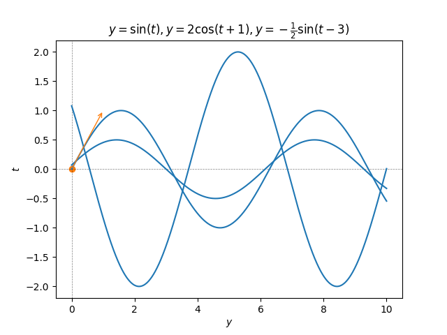
Adding constraints to the ODE translates to constraints on the amplitude and phase shift. For instance \[x''(t)+x(t)=0,\quad\quad x(0)=0,x'(0)=1,\tag{5.38}\] can be solved starting with the form \(x(t)=\alpha\cos(t)+\beta\sin(t)\) of the general solution and noting that then \(x(0)=\alpha\cos(0)+\beta\sin(0)=\alpha\) and \(x'(0)=-\alpha\sin(0)+\beta\cos(0)=\beta,\) so the IVP ([eq:ch5_so_lin_aut_cos_sin_IVP]) is solved by \[x(t)=\sin(t).\] This and a few other solutions are showed in the next figure.
(Characteristic equation with purely imaginary roots II) Consider the ODE \[x''(t)+3x(t)=0,\] with characteristic polynomial \[r^{2}+3=0,\] with purely imaginary roots \(\pm\sqrt{3}i.\) Making the trigonometric ansatz \[x(t)=\cos(\omega t+s)\] as before we compute \(x''(t)=-\omega^{2}\cos(\omega x+s)\) and plug in to obtain \[-\omega^{2}\cos(\omega t+s)+3\cos(\omega t+s)=0.\] This holds identically iff \(\omega=\pm\sqrt{3}\) so \[x(t)=\alpha\cos(\sqrt{3}t+s),\:\alpha\in\mathbb{R},s\in\mathbb{R},\] is a family of solutions, which could also be written as \[x(t)=\alpha\sin(\sqrt{3}t+s),\:\alpha\in\mathbb{R},s\in\mathbb{R},\] or \[x(t)=\alpha\cos(\sqrt{3}t)+\beta\sin(\sqrt{3}t),\alpha,\beta\in\mathbb{R}.\] These solutions are sinusoids of frequency \(\sqrt{3}\) and any amplitude or phase.
The more general ODE \[x''(t)+Lx(t)=0\quad\quad\quad\text{with}\quad\quad L>0\tag{5.40}\] has characteristic equation \(r^{2}+L=0\) with purely imaginary roots \(\pm i\sqrt{L}\) and it is not hard to see that the sinusoids with frequency \(\sqrt{L}\) and any amplitude and phase are a family of solutions, which can be variously written as \[x(t)=\alpha\cos(\sqrt{L}t+s),\quad\alpha,s\in\mathbb{R},\tag{5.41}\] \[x(t)=\alpha\sin(\sqrt{L}t+s),\quad\alpha,s\in\mathbb{R},\tag{5.42}\] \[x(t)=\alpha\cos(\sqrt{L}t)+\beta\sin(\sqrt{L}t),\quad\alpha,\beta\in\mathbb{R}.\tag{5.43}\] Below we will prove that these sinusoids are actually all the solutions of the equation ([eq:ch5_so_lin_aut_pure_imag_roots_general]).
\(\text{ }\) Complex solutions. Recall that \(e^{i\theta}=\cos(\theta)+i\sin(\theta)\) and \[\cos(\theta)=\frac{e^{i\theta}+e^{-i\theta}}{2}\quad\quad\sin(\theta)=\frac{e^{i\theta}-e^{-i\theta}}{2i}.\tag{5.44}\] Thus the solutions ([eq:ch5_so_lin_aut_pure_imag_roots_general_sols_sin_cos]) of ([eq:ch5_so_lin_aut_pure_imag_roots_general]) can be written as \[\alpha\frac{e^{i\sqrt{L}t}+e^{-i\sqrt{L}t}}{2}+\beta\frac{e^{i\sqrt{L}t}-e^{-i\sqrt{L}t}}{2i}=\frac{\alpha+\beta}{2}e^{i\sqrt{L}t}+\frac{\alpha-\beta}{2i}e^{-i\sqrt{L}t}.\] Note that the roots of the characteristic equation in this case are \(r_{1}=i\sqrt{L},r_{1}=-i\sqrt{L}\) so this can be written as \[\alpha e^{r_{1}t}+\beta e^{r_{2}t}\] for modified constants \(\alpha,\beta\in\mathbb{C}.\) At the level of notation this is identical to the general form of the solutions ([eq:ch5_so_lin_aut_real_roots_all_sols_hom_ODE_sols]) when the roots \(r_{1},r_{2}\) are distinct real! This suggests that even when \(r_{1}\) is complex \(e^{r_{1}t}\) is a solution to the ODE. But what does this even mean when \(r_{1}\) is complex?
The following definitions make sense of this.
If \(I\) is an interval we say that a function \(y:I\to\mathbb{C}\) is differentiable if it is differentiable as a map from \(I\to\mathbb{R}^{2}\) (identifying \(\mathbb{R}^{2}\) and \(\mathbb{C}\)) and we define its derivative as \(y'(t)=\frac{d}{dt}\mathrm{Re}y(t)+i\frac{d}{dt}{\rm Im}y(t).\)
If \(y\) actually takes only real values then \(y'(t)\) as defined above coincides with the usual real derivative. With this definition of derivative of a complex values function the usual derivation rules hold. For instance if \(z:I\to\mathbb{C}\) is differentiable and \(f:\mathbb{C}\to\mathbb{C}\) is differentiable in the complex analytic sense (i.e. holomorphic) then \[\frac{d}{dt}f(z(t))=f'(z(t))z'(t).\] We will actually only use this with \(f(z)=e^{rz},\) in which one can also check directly from the definition of \(z'(t)\) and complex multiplication in terms of real and imaginary part that \[\frac{d}{dt}f(z(t))=re^{rz(t)}z'(t).\tag{5.46}\]
(\(\mathbb{C}\)-valued first and second order linear autonomous ODEs). For any non-empty interval \(I\) and \(a,b\in\mathbb{C}\) we call \[y=ay'+b,\quad\quad t\in I,\tag{5.47}\] a first order linear autonomous complex ODE, and any differentiable function \(y:I\to\mathbb{C}\) for which ([eq:ch5_def_complex_fo_lin_aut]) holds is a solution to the ODE.
For any \(a_{1},a_{0},b\in\mathbb{C}\) we call \[y''+a_{1}y'+a_{0}y=b,\quad\quad t\in I,\tag{5.48}\] a second order linear autonomous complex ODE, if \(b=0\) we additionally call it homogeneous, and any differentiable function \(y:I\to\mathbb{C}\) for which ([eq:ch5_def_complex_so_lin_aut]) holds is a solution to the ODE.
We call the quadratic \[r^{2}+a_{1}r+a_{0}\tag{5.49}\] in the complex variable \(r\) the characteristic polynomial of ([eq:ch5_def_complex_so_lin_aut]).
Let \(a_{0},a_{1},b\in\mathbb{R}\) and \(I\) be a non-empty interval.
a) Assume \(a_{0}\ne0.\) Then a a function \(y\) is a solution to ([eq:ch5_so_lin_aut_gen]) iff \(x=y-\frac{b}{a_{0}}\) is a solution to ([eq:ch5_so_lin_aut_homo_def]).
b) \(y(t)=0\) is a solution to ([eq:ch5_so_lin_aut_homo_def]).
c) If \(y\) is a solution to ([eq:ch5_so_lin_aut_homo_def]) then \(\alpha y\) is also a solution for any \(\alpha\in\mathbb{R}.\)
d) If \(y_{1}\) and \(y_{2}\) are solutions to ([eq:ch5_so_lin_aut_homo_def]) then \(y_{1}+y_{2}\) is also a solution to ([eq:ch5_so_lin_aut_homo_def]).
If \(I\) is an interval we say that a function \(y:I\to\mathbb{C}\) is differentiable if it is differentiable as a map from \(I\to\mathbb{R}^{2}\) (identifying \(\mathbb{R}^{2}\) and \(\mathbb{C}\)) and we define its derivative as \(y'(t)=\frac{d}{dt}\mathrm{Re}y(t)+i\frac{d}{dt}{\rm Im}y(t).\)
If \(I\) is an interval we say that a function \(y:I\to\mathbb{C}\) is differentiable if it is differentiable as a map from \(I\to\mathbb{R}^{2}\) (identifying \(\mathbb{R}^{2}\) and \(\mathbb{C}\)) and we define its derivative as \(y'(t)=\frac{d}{dt}\mathrm{Re}y(t)+i\frac{d}{dt}{\rm Im}y(t).\)
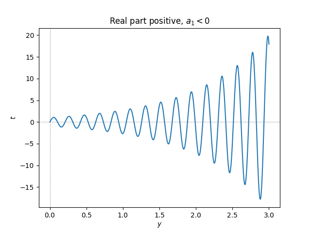
\(\text{ }\) Imaginary roots with non-zero real part Consider now the ODE \[x''+a_{1}x'+a_{0}x=0,\tag{5.50}\] with real coefficients \(a_{1},a_{0}\) such that \(a_{1}^{2}-4a_{0}<0,\) so that the characteristic equation ([eq:ch5_so_lin_aut_homo_imag_root_nonzero_real_part]) of has solutions \[r_{1}=v+i\omega\quad\quad r_{2}=v-i\omega\] for \(v,\omega\in\mathbb{R},v\ne0,w\ne0.\) Viewing ([eq:ch5_so_lin_aut_homo_imag_root_nonzero_real_part]) as a complex ODE we see as above that \[x(t)=e^{vt+i\omega t}\quad\quad\quad x(t)=e^{vt-i\omega t}\] are complex solutions, so \[\frac{e^{vt+i\omega t}+e^{vt-i\omega t}}{2}=e^{vt}\cos(\omega t),\tag{5.51}\] and \[\frac{e^{vt+i\omega t}-e^{vt-i\omega t}}{2i}=e^{vt}\sin(\omega t)\tag{5.52}\] also solutions. But the r.h.s.s. of ([eq:ch5_so_lin_aut_homo_imag_root_nonzero_real_part_cos_sol]) and ([eq:ch5_so_lin_aut_homo_imag_root_nonzero_real_part_sin_sol]) are real, so these are also real solutions to the ODE ([eq:ch5_so_lin_aut_homo_imag_root_nonzero_real_part]).
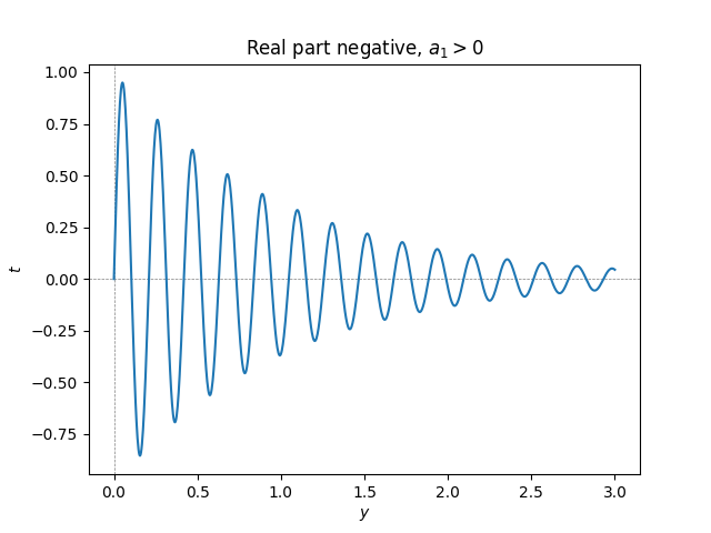
Taking linear combinations of ([eq:ch5_so_lin_aut_homo_imag_root_nonzero_real_part_cos_sol]) and ([eq:ch5_so_lin_aut_homo_imag_root_nonzero_real_part_sin_sol]) and using trigonometric identities we see that \[\alpha e^{vt}\cos(\omega t+s),\alpha,s\in\mathbb{R},\quad\alpha e^{vt}\sin(\omega t+s),\alpha,s\in\mathbb{R},\quad e^{vt}\left\{ \alpha\cos(\omega t)+\beta\sin(\omega t)\right\} ,\alpha,\beta\in\mathbb{R},\tag{5.54}\] are three equivalent ways of writing these solutions to ([eq:ch5_so_lin_aut_homo_imag_root_nonzero_real_part]), cf. ([eq:ch5_so_lin_aut_pure_imag_roots_general_sols_cos])-([eq:ch5_so_lin_aut_pure_imag_roots_general_sols_sin_cos]). These solutions are sinusoids with exponentially growing or exponentially decaying magnitude. The magnitude is growing if \(v>0,\) i.e. \(a_{1}<0,\) and decaying if \(v<0,\) i.e. \(a_{1}>0.\)
With the machinery of complex ODEs and complex solutions we can now prove the existence and uniqueness of solutions.
Assume \(a,b\in\mathbb{C},\) \(a\ne0,\) \(I\subset\mathbb{R}\) an interval. Then a complex differentiable function \(y:I\to\mathbb{C}\) is a solution to \[\dot{y}(t)=ay(t)+b\quad t\in I,\tag{5.57}\] iff \(y(t)=\alpha e^{at}-\frac{b}{a}\) for some \(\alpha\in\mathbb{C}.\) For any \(t_{*}\in I\) and \(y_{0}\in\mathbb{C}\) the same ODE subject to the constraint \[y(t_{*})=y_{0},\tag{5.58}\] has the unique solution \[y(t)=\left(y_{0}+\frac{b}{a}\right)e^{a(t-t_{*})}-\frac{b}{a}\quad\forall t\in I.\tag{5.59}\]
(Complete solution of first order autonomous ODEs with \(a\ne0\)). Assume \(a,b\in\mathbb{R},a\ne0\) and \(I\subset\mathbb{R}\) an interval. Then a function \(y(t)\) is a solution of the ODE \[\dot{y}(t)=ay(t)+b,\quad\quad t\in I,\tag{3.23}\] iff \[y(t)=\alpha e^{at}-\frac{b}{a}\quad\forall t\in I,\text{ for some }\alpha\in\mathbb{R}.\tag{3.24}\]
(Uniqueness second order complex linear autonomous ODE) Let \(I\) be a non-empty interval. Let \(a_{1},a_{0}\in\mathbb{C}.\) Consider the complex second order linear autonomous ODE \[x''+a_{1}x'+a_{0}x=0,\quad\quad t\in I.\tag{5.60}\] Let \(r_{1},r_{2}\in\mathbb{C},r_{1}\ne r_{2}\) denote the two roots of its characteristic equation \[r^{2}+a_{1}r+a_{2}r=0.\tag{5.61}\]
a) A function \(x\) solves the ODE ([eq:ch5_so_lin_aut_char_eq_gen]) iff \[x(t)=\alpha_{1}e^{r_{1}t}+\alpha_{2}e^{r_{2}t},\tag{5.62}\] for some \(\alpha_{1},\alpha_{2}\in\mathbb{\mathbb{C}}.\)
b) For any \(t_{0}\in I\) and \(x_{0},x_{1}\in\mathbb{C},\) a function \(y\) solves the constrained homogeneous ODE \[x''+a_{1}x'+a_{0}=0,\quad\quad t\in I,x(t_{0})=x_{0},x'(t_{0})=x_{1},\tag{5.63}\] iff \[x(t)=\frac{-x_{0}r_{2}+x_{1}}{r_{1}-r_{2}}e^{r_{1}(t-t_{0})}+\frac{x_{0}r_{1}-x_{1}}{r_{1}-r_{2}}e^{r_{2}(t-t_{0})}.\tag{5.64}\]
c) If \(b\in\mathbb{R}\) and \(a_{0}\ne0\) a function \(y\) solves the non-homogeneous second order autonomous ODE \[y''+a_{1}y'+a_{0}y=b,\quad\quad t\in I,\tag{5.65}\] iff \[y(t)=\alpha_{1}e^{r_{1}t}+\alpha_{2}e^{r_{2}t}+\frac{b}{a_{0}},\quad\quad t\in I\] and if \(t_{0}\in I,y_{0},y_{1}\in\mathbb{C}\) then a function \(y\) solves the constrained non-homogeneous second order autonomous ODE \[y(t)=\alpha_{1}e^{r_{1}t}+\alpha_{2}e^{r_{2}t}+\frac{b}{a_{0}},\quad\quad t\in I,y(t_{0})=y_{0},y'(t_{0})=y_{1}\] iff \[y(t)=\frac{-\left(x_{0}-\frac{b}{a_{0}}\right)r_{2}+x_{1}}{r_{1}-r_{2}}e^{r_{1}(t-t_{0})}+\frac{\left(x_{0}-\frac{b}{a_{0}}\right)r_{1}-x_{1}}{r_{1}-r_{2}}e^{r_{2}(t-t_{0})}+\frac{b}{a_{0}},\quad\quad t\in I.\]
(Uniqueness: distinct real roots). Let \(I\) be a non-empty interval, and \(a_{1},a_{0}\in\mathbb{R}\) such that \(a_{1}^{2}-4a_{0}>0.\) Consider the second order linear autonomous ODE \[x''+a_{1}x'+a_{0}x=0,\quad\quad t\in I.\tag{5.23}\] Let \(r_{1},r_{2}\in\mathbb{R},r_{1}\ne r_{2}\) denote the two roots of its characteristic equation \[r^{2}+a_{1}r+a_{0}=0.\tag{5.24}\]
a) [Homogeneous] A function \(x\) solves the ODE ([eq:ch5_so_lin_aut_real_roots_all_sols_hom_ODE]) iff \[x(t)=\alpha_{1}e^{r_{1}t}+\alpha_{2}e^{r_{2}t},\tag{5.25}\] for some \(\alpha_{1},\alpha_{2}\in\mathbb{R}.\)
b) [Constrained Homogeneous] For any \(t_{0}\in I\) and \(x_{0},x_{1}\in\mathbb{R},\) a function \(y\) solves \[x''(t)+a_{1}x'(t)+a_{0}=0,\quad\quad t\in I,\quad\quad x(t_{0})=x_{0},x'(t_{0})=x_{1},\tag{5.26}\] iff \[x(t)=\frac{-x_{0}r_{2}+x_{1}}{r_{1}-r_{2}}e^{r_{1}(t-t_{0})}+\frac{x_{0}r_{1}-x_{1}}{r_{1}-r_{2}}e^{r_{2}(t-t_{0})}.\tag{5.27}\]
c) [Non-homogeneous] If \(b\in\mathbb{R}\) and \(a_{0}\ne0\) then a function \(y\) solves \[y''+a_{1}y'+a_{0}y=b,\quad\quad t\in I,\tag{5.28}\] iff \[y(t)=\alpha_{1}e^{r_{1}t}+\alpha_{2}e^{r_{2}t}+\frac{b}{a_{0}},\quad\quad t\in I.\]
d) [Non-homogeneous constrained] If in addition \(t_{0}\in I,y_{0},y_{1}\in\mathbb{R}\) then a function \(y\) solves \[y''(t)+a_{1}y'(t)+a_{0}y(t)=b\quad\quad t\in I,y(t_{0})=y_{0},y'(t_{0})=y_{1}\] iff \[y(t)=\frac{-\left(y_{0}-\frac{b}{a_{0}}\right)r_{2}+y_{1}}{r_{1}-r_{2}}e^{r_{1}(t-t_{0})}+\frac{\left(y_{0}-\frac{b}{a_{0}}\right)r_{1}-y_{1}}{r_{1}-r_{2}}e^{r_{2}(t-t_{0})}+\frac{b}{a_{0}},\quad\quad t\in I.\]
(Complete solution of first order autonomous ODEs with \(a\ne0\)). Assume \(a,b\in\mathbb{R},a\ne0\) and \(I\subset\mathbb{R}\) an interval. Then a function \(y(t)\) is a solution of the ODE \[\dot{y}(t)=ay(t)+b,\quad\quad t\in I,\tag{3.23}\] iff \[y(t)=\alpha e^{at}-\frac{b}{a}\quad\forall t\in I,\text{ for some }\alpha\in\mathbb{R}.\tag{3.24}\]
Assume \(a,b\in\mathbb{C},\) \(a\ne0,\) \(I\subset\mathbb{R}\) an interval. Then a complex differentiable function \(y:I\to\mathbb{C}\) is a solution to \[\dot{y}(t)=ay(t)+b\quad t\in I,\tag{5.57}\] iff \(y(t)=\alpha e^{at}-\frac{b}{a}\) for some \(\alpha\in\mathbb{C}.\) For any \(t_{*}\in I\) and \(y_{0}\in\mathbb{C}\) the same ODE subject to the constraint \[y(t_{*})=y_{0},\tag{5.58}\] has the unique solution \[y(t)=\left(y_{0}+\frac{b}{a}\right)e^{a(t-t_{*})}-\frac{b}{a}\quad\forall t\in I.\tag{5.59}\]
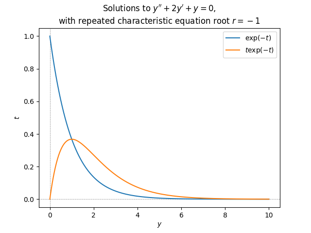
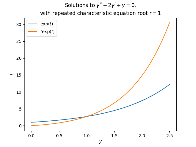
\(\text{ }\) Repeated root We have now found all solutions to second order linear autonomous equations whose characteristic equation as distinct roots (whether they are real or complex - including if the ODE has complex coefficients and/or initial conditions). But our results break down when \(\rho=r_{1}=r_{2},\) i.e. when the characteristic polynomial is \[(r-\rho)^{2}=r^{2}+\underset{=a_{1}}{\underbrace{(-2r)}}\rho+\underset{=a_{0}}{\underbrace{\rho^{2}}.}\tag{5.66}\] In this we do have that \(y(t)=e^{\rho t}\) is a solution to the homogeneous equation, but we don’t have a second solution of this form since \(r_{1}=r_{2}.\) Also for instance the argument ([eq:ch5_so_lin_aut_real_roots_all_sols_matrix_vec]) breaks down. However, a close inspection of ([eq:ch5_so_lin_aut_real_roots_all_sols_z_comp_start])-([eq:ch5_so_lin_aut_real_roots_all_sols_z_comp_start]) shows that that argument doesn’t depend on \(r_{1}\ne r_{2}.\) The identity ([eq:ch5_so_lin_aut_real_roots_z_fo_ODE]) with \(r_{1}=r_{2}\) proves that for any solution \(y(t)\) it holds that \[\frac{d^{2}}{dt^{2}}\left\{ e^{-\rho t}y(t)\right\} =0,\] which implies that \[\frac{d}{dt}\left\{ e^{-\rho t}y(t)\right\} =c,\] for some constant \(c,\) which then in turns implies that \[e^{-\rho t}y(t)=a+ct\] for some \(a,c\in\mathbb{C}.\) This is equivalent to \[y(t)=ae^{\rho t}+cte^{\rho t}.\] The term \(ae^{\rho t}\) is the solution we already have, but \(cte^{\rho t}\) is new. We can use it as ansatz to double-check if this is a solution: If \(y(t)=te^{\rho t}\) then \(y'(t)=e^{\rho t}+\rho te^{\rho t}\) and \(y''(t)=2\rho e^{\rho t}+\rho^{2}te^{\rho t},\) so \[\begin{array}{l} y''+a_{1}y'+a_{0}\\ =2\rho e^{\rho t}+\rho^{2}te^{\rho t}+a_{1}\left(e^{\rho t}+\rho te^{\rho t}\right)+a_{0}te^{\rho t}\\ =e^{\rho t}t\left(\rho^{2}+a_{1}\rho+a_{0}\right)+\left(2\rho+a_{1}\right)e^{\rho t}. \end{array}\tag{5.67}\] Since \(\rho\) is a solution to the characteristic equation \(\rho^{2}+a_{1}\rho+a_{0}=0,\) so the first term vanishes. The second term also vanishes due to the form of \(a_{1}\) for these ODEs, from ([eq:ch5_so_lin_aut_repeated_root]). Thus indeed \(te^{\rho t}\) is a solution, and so is then any linear combination \(\alpha e^{\rho t}+\beta te^{\rho t}.\) When the coefficients \(a_{1},a_{0}\) are real the repeated root is also real, and then \(te^{\rho t}\) is a term that for small \(t\) is close to zero - unlike \(e^{\rho t}\) - and for large \(t\) decays to zero slightly slower than \(e^{\rho t}\) if \(\rho<0\) or grows slightly faster if \(\rho>0.\)
We finish with the proof that these are all the solutions for these ODEs.
(Uniqueness second order complex linear autonomous ODE with repeated characteristic polynomial root) Let \(I\) be a non-empty interval. Let \(a_{1},a_{0}\in\mathbb{C}\) be s.t. the two roots of its characteristic equation \[r^{2}+a_{1}r+a_{0}r=0,\tag{5.68}\] has a repeated non-zero root, i.e. \(a_{1}^{2}-4a_{0}=0,a_{0}\ne0.\) Write \(\rho=-\frac{a_{1}}{2}\) for the repeated root. Consider the complex second order linear autonomous ODE \[x''+a_{1}x'+a_{0}x=0,\quad\quad t\in I.\tag{5.69}\]
a) A function \(x\) solves the ODE ([eq:ch5_so_lin_aut_char_eq_gen]) iff \[x(t)=\alpha_{1}e^{\rho t}+\alpha_{2}te^{\rho t},\tag{5.70}\] for some \(\alpha_{1},\alpha_{2}\in\mathbb{\mathbb{C}}.\)
b) For any \(t_{0}\in I\) and \(x_{0},x_{1}\in\mathbb{C},\) a function \(y\) solves the constrained homogeneous ODE \[x''+a_{1}x'+a_{0}=0,\quad\quad t\in I,x(t_{0})=x_{0},x'(t_{0})=x_{1},\tag{5.71}\] iff \[x(t)=x_{0}e^{\rho(t-t_{0})}+\left(x_{1}-x_{0}\right)\frac{t-t_{0}}{\rho}e^{\rho(t-t_{0})}.\tag{5.72}\]
c) If \(b\in\mathbb{R}\) and \(a_{0}\ne0\) a function \(y\) solves the non-homogeneous second order autonomous ODE \[y''+a_{1}y'+a_{0}y=b,\quad\quad t\in I,\tag{5.73}\] iff \[y(t)=\alpha_{1}e^{r_{1}t}+\alpha_{2}e^{r_{2}t}+\frac{b}{a_{0}},\quad\quad t\in I\] and if \(t_{0}\in I,y_{0},y_{1}\in\mathbb{C}\) then a function \(y\) solves the constrained non-homogeneous second order autonomous ODE \[y(t)=\alpha_{1}e^{r_{1}t}+\alpha_{2}e^{r_{2}t}-\frac{b}{a_{0}},\quad\quad t\in I,y(t_{0})=y_{0},y'(t_{0})=y_{1}\] iff \[y(t)=\frac{-\left(x_{0}-\frac{b}{a}\right)r_{2}+x_{1}}{r_{1}-r_{2}}e^{r_{1}(t-t_{0})}+\frac{\left(x_{0}-\frac{b}{a}\right)r_{1}-x_{1}}{r_{1}-r_{2}}e^{r_{2}(t-t_{0})}+\frac{b}{a_{0}},\quad\quad t\in I.\]
(Complete solution of first order autonomous ODEs with \(a\ne0\)). Assume \(a,b\in\mathbb{R},a\ne0\) and \(I\subset\mathbb{R}\) an interval. Then a function \(y(t)\) is a solution of the ODE \[\dot{y}(t)=ay(t)+b,\quad\quad t\in I,\tag{3.23}\] iff \[y(t)=\alpha e^{at}-\frac{b}{a}\quad\forall t\in I,\text{ for some }\alpha\in\mathbb{R}.\tag{3.24}\]
It only remains to prove that there is a unique solution to ([eq:ch5_so_lin_aut_real_roots_all_sols_IVP-1-1-1]) of the form ([eq:ch5_so_lin_aut_real_roots_all_sols_hom_ODE_sols-1-1-1]). This follows since if \(x\) has the form ([eq:ch5_so_lin_aut_real_roots_all_sols_hom_ODE_sols-1-1-1]) then \[x'(t)=\alpha_{1}\rho e^{\rho t}+\alpha_{2}t\rho e^{\rho t}+\alpha_{2}e^{\rho t},\] so the constraints are equivalent to \[\begin{array}{lcl} \alpha_{1}e^{\rho t_{0}}+\alpha_{2}t_{0}e^{\rho t_{0}} & = & x_{0},\\ \alpha_{1}\rho e^{\rho t_{0}}+\alpha_{2}\rho t_{0}e^{\rho t_{0}}+\alpha_{2}e^{\rho t_{0}} & = & x_{1}, \end{array}\tag{5.74}\] i.e. \[\left(\begin{matrix}e^{\rho t_{0}} & t_{0}e^{\rho t_{0}}\\ \rho e^{\rho t_{0}} & \rho t_{0}e^{\rho t_{0}}+e^{\rho t_{0}} \end{matrix}\right)\left(\begin{matrix}\alpha_{1}\\ \alpha_{2} \end{matrix}\right)=\left(\begin{matrix}x_{0}\\ x_{1} \end{matrix}\right).\] The matrix has determinant \[e^{\rho t_{0}}\left(\rho t_{0}e^{\rho t_{0}}+e^{\rho t_{0}}\right)-t_{0}\rho e^{2\rho t_{0}}=e^{2\rho t_{0}}\ne0,\] so the system ([eq:ch5_so_lin_aut_real_roots_all_sols_complex_repeated_root_constraint_system]) has a unique solution, and thus the constrained ODE ([eq:ch5_so_lin_aut_real_roots_all_sols_IVP-1-1-1]) has a unique solution. Since it is easily verified that ([eq:ch5_so_lin_aut_real_roots_all_sols_IVP_sol-1-1-1]) is a solution it must be this unique solution.
5.2 Idealized spring-mass system - harmonic oscillator
In this section we investigate a very important application of the second order linear autonomous ODE: modelling an idealized spring with a mass attached. Here is a diagram of the system:
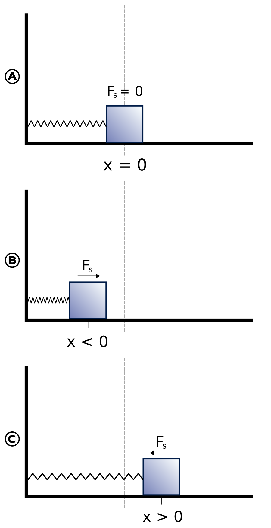
\(\text{ }\) Deriving the ODE A mass attached to a spring is subject to Newton’s second law \(f=ma,\) which we encountered in Section 1.1. Let \(y(t)\) denote the position of the mass at time \(t,\) where \(y(t)=0\) if the spring is neither compressed nor extended but in a neutral position (A in the diagram), while \(y(t)>0\) if the spring is stretched (C in the diagram) and \(y(t)<0\) if the spring is compressed (B in the diagram). Then \(y'(t)\) is the velocity of the mass, and \(y''(t)\) is the acceleration. Thus by Newton’s second law \[y''(t)=\frac{f_{{\rm tot}}}{m},\tag{5.76}\] where \(f_{{\rm tot}}\) denotes the net force on the mass. Let us for simplicity assume \(m=1.\) The force due to the tension of the spring is modelled by Hooke’s law, stating that the force the spring exerts on the mass is approximately proportional to the displacement away from the neural position, i.e. \[f_{{\rm spring}}=-ky(t),\] for a constant \(k\in\mathbb{R},k>0.\) Furthermore the spring may be subject to friction which we model as \[f_{{\rm fric}}=-\gamma y'(t).\] Taking into account these forces we arrive at the ODE model \[y''(t)+\gamma y'(t)+ky(t)=0.\tag{5.77}\]
\(\text{ }\) Stationary solution Recall from the previous section that this ODE with the constraints \(y(0)=y_{0}\) and \(y'(0)=y_{1}\) has a unique solution. Therefore if the spring starts in a neutral position (\(y(0)=0\)) and is at rest \((y'(0)=0\)) then stationary solution \(y(t)=0\) is the unique solution, with the interpretation that the spring remains neutral and at rest for all \(t\ge0\) in this scenario.
\(\text{ }\) Without friction - undamped case. Let us assume that there is no friction, i.e. \(\gamma=0.\) This is called an undamped spring. Then the ODE reduces to \[y''(t)+ky(t)=0.\tag{5.78}\] By the results of the previous section all solutions of this ODE are of the form \[y(t)=\alpha\cos(\sqrt{k}t+s),\tag{5.79}\] i.e. sinusoids of frequency \(\sqrt{k}\) and any amplitude and phase. If we for instance assume that the spring is initially compressed a distance of \(1\) length units, so that \(y(0)=-1,\) and released from there from rest so that \(y'(0)=0,\) we should impose the initial conditions \[y(0)=-1\text{ and }y'(0)=0.\tag{5.80}\] Since \(y'(t)=\alpha\sin(\sqrt{k}t+s)\) so \(y'(0)=\alpha\sqrt{k}\sin(s)=0\) if \(s=0,\) while \(y(0)=\alpha\cos(s)=-1\) if \(s=0,\alpha=-1,\) we obtain the solution \[y(t)=-\cos(\sqrt{k}t),\tag{5.81}\] which is plotted in this figure:
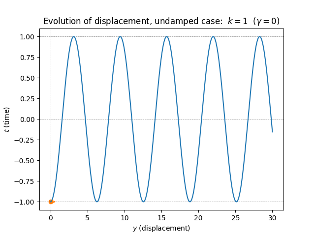
This solution, and indeed the solution for any non-trivial initial conditions, is a non-decaying perfectly periodic sinusoid. The absence of decay reflects our assumption of no friction, which means no energy is lost and the oscillation can continue forever once started. Since all the energy is preserved the spring attains the same maximum compression and extension in each period of the oscillation. The larger the initial displacement, and/or the larger the initial velocity back towards neural, the higher the amplitude of the oscillation. The frequency of the oscillation is however determined purely by the coefficient \(k.\)
\(\text{ }\) Small positive friction - underdamped. Now let us consider the case of positive but weak friction. Now the ODE has the form \[y''(t)+\gamma y'(t)+ky(t)=0.\tag{5.82}\] Recall from the previous section that the behavior of the solutions of this ODE depends greatly on whether the roots of the characteristic equation \[r^{2}+\gamma r+k=0,\tag{5.83}\] are real/complex and distinct/repeated. For \(\gamma>0\) very small the solutions will be complex and distinct, and this will be the case as long as \[0<\gamma<2\sqrt{k}.\tag{5.84}\] When this holds the roots of the characteristic polynomial is \[-\frac{1}{2}\gamma\pm i\omega\quad\quad\text{ where }\quad\quad\omega=\frac{1}{2}\sqrt{4k-\gamma^{2}},\] and solutions are of the form \[y(t)=e^{-\frac{\gamma}{2}t}\left\{ \alpha\cos(\omega t)+\beta\sin(\omega t)\right\} ,\tag{5.85}\] (we use this form instead of just cos with a phase shift \(s,\) since it makes it easier to solve for the initial conditions). Note that the frequency of oscillation is given by \[\omega=\frac{1}{2}\sqrt{4k-\gamma^{2}}<\sqrt{k},\] which means it is somewhat lower than the frequency in the undamped case \(\gamma=0,\) which is \(\sqrt{k}.\)
Let us imagine the same initial conditions as before, namely starting with a spring compressed \(1\) length unit and at rest, i.e. satisfying ([eq:ch5_aut_spring_mass_undamped_ODE_IVP]). Now \(y(0)=\alpha e^{-\frac{\gamma}{2}\cdot0}\cos(\sqrt{\omega}\cdot0)=\alpha,\) so the first constraint forces \(\alpha=-1.\) On the other hand \[y'(t)=-\frac{\gamma}{2}e^{-\frac{\gamma}{2}t}\left\{ \alpha\cos(\omega t)+\beta\sin(\omega t)\right\} +e^{-\frac{\gamma}{2}t}\sqrt{\omega}\left\{ -\alpha\sin(\omega t)+\beta\cos(\omega t)\right\} ,\] so \(y'(0)=-\frac{\gamma}{2}\alpha+\sqrt{\omega}\beta\) and the second constraint forces \(\beta=\frac{\gamma\alpha}{2\omega}=-\frac{\gamma}{2\omega},\) so the unique constrained solution is \[y(t)=e^{-\frac{\gamma}{2}t}\left\{ -\cos(\omega t)-\frac{\gamma}{2\omega}\sin(\omega t)\right\} .\] This solution is plotted for different \(\gamma>0\) in the following figure.
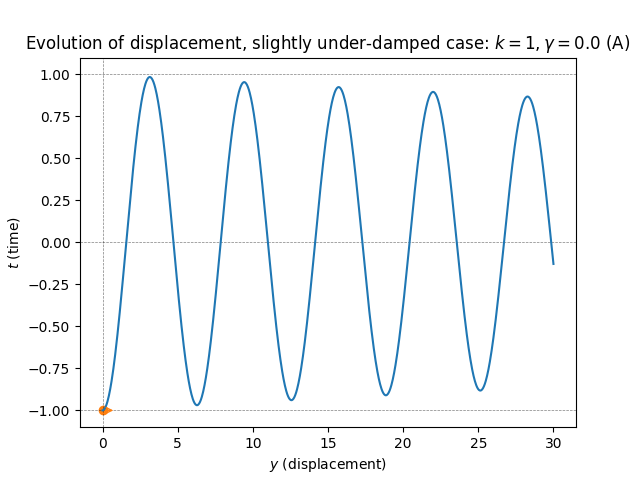
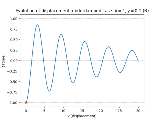
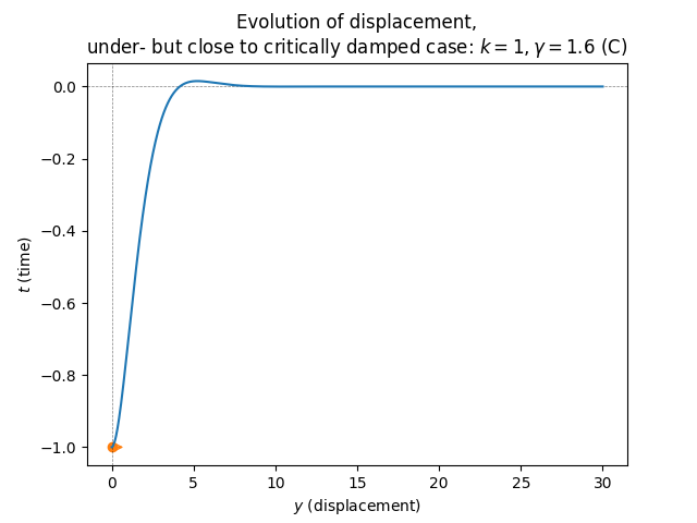
These solutions are decaying sinusoids. The amplitude decreases exponentially as \(t\to\infty.\) This reflect that the system now loses energy due to friction/damping as it oscillates.
If \(\gamma\) is positive but very small the decay of the amplitude is very slow, and for \(\gamma\downarrow0\) one approaches the solutions of the undamped case (plot A).
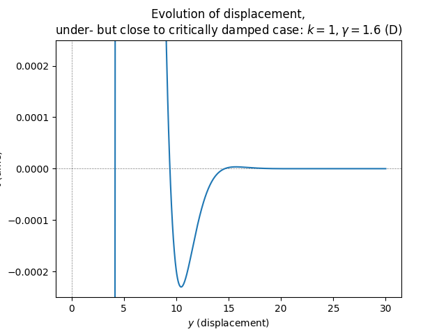
If \(\gamma\) is below \(2\sqrt{k}\) but very close to it, the oscillation decays very fast, and becomes almost imperceptible after only a few periods (plot C). The frequency is also reduced, tending to zero as \(\gamma\uparrow2\sqrt{k}.\) Still, the solution does cross the neutral position \(y=0\) an infinite number of times, as one can be seen by zooming in (plot D).
In between the extremes is the canonical underdamped behavior, where the amplitude of the oscillation decays at a steady but not extreme rate, and the frequency is reduced but not massively so (plot B).
\(\text{ }\) Strong friction - overdamped. From the previous section we know that if \[\frac{\gamma^{2}}{4}>k\text{ and }\gamma>0\] then the characteristic equation has negative real roots which equal \[r_{1}=-\frac{\gamma-\sqrt{\gamma^{2}-4k}}{2}\text{ and }r_{2}=-\frac{\gamma+\sqrt{\gamma^{2}-4k}}{2}.\] The general solution is \[y(t)=\alpha e^{r_{1}t}+\beta e^{r_{2}t}\tag{5.87}\] representing exponentially decaying displacement (at two different rates: the term \(e^{-r_{1}t}\) decays faster). With the initial conditions ([eq:ch5_spring_aut_underdamped_ODE_gamma_cond]) the unique solution is \[y(t)=-\frac{r_{2}}{r_{2}-r_{1}}e^{r_{1}t}+\frac{r_{1}}{r_{2}-r_{1}}e^{r_{2}t}.\tag{5.88}\]
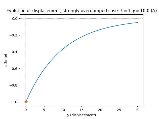
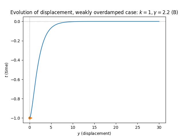
There is no oscillation, and the displacement simply decays exponentially. For \(\gamma\) closer to the threshold \(2\sqrt{k}\) the rate of decrease is faster (plot B), while for \(\gamma\) very large the large friction causes the decay to slow down (plot A).
\(\text{ }\) Critical friction - critically damped. On the boundary between the overdamped and underdamped regions is the critically damped region, where: \[\gamma=2\sqrt{k}\] In this case the characteristic polynomial has the repeated real root \(r=\frac{\gamma}{2}.\) In this case the general solution is of the form \[y(t)=\alpha e^{-\frac{\gamma}{2}t}+\beta te^{-\frac{\gamma}{2}t}.\tag{5.89}\] The initial conditions are satisfied by \[y(t)=-e^{-\frac{\gamma}{2}t}-\frac{\gamma}{2}te^{-\frac{\gamma}{2}t}.\]
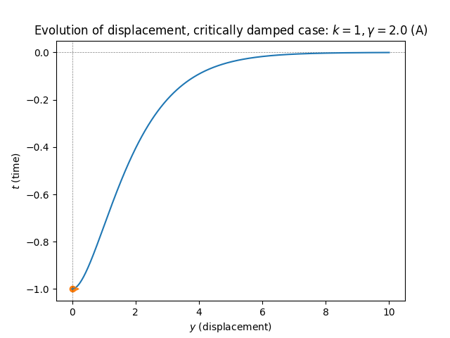
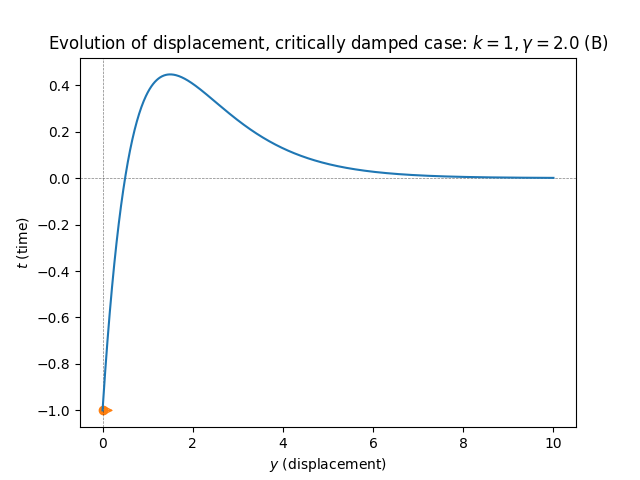
In this case the displacement simply decays - at a slower rate than in the overdamped case, but fast enough to prevent oscillation (plot A). However if the initial condition provides enough energy, e.g. by not starting at rest but rather at a positive velocity such as \(y'(0)=\frac{3}{3}\gamma,\) the displacement can cross the axis exactly \(y=0\) once, before settling in to a monotonic decay towards the neural position \(y=0\) (plot B).
5.3 \(k\ge3\)-th order linear autonomous equations
If \(I\) is a non-empty interval, \(k\ge1\) and \(a_{0},\ldots,a_{k-1},b\in\mathbb{R}\) we call the ODE ([eq:ch5_higher_order_lin_aut]) a \(k\)-th order linear autonomous ODE, or equivalently a \(k\)-th order linear ODE with constant coefficients.
(Order \(k\) linear autonomous ODE) Let \(I\) be a non-empty interval, let \(k\ge1\) and \(a_{0},\ldots,a_{k-1},b\in\mathbb{C}.\) The ODE of the form \[y^{(k)}+\sum_{l=0}^{k-1}a_{l}y^{(l)}=b,\quad\quad t\in I.\tag{5.91}\] is called a \(k\)-th order linear autonomous equation, or equivalently a \(k\)-th order linear ODE with constant coefficients. We call \[y^{(k)}+\sum_{l=0}^{k-1}a_{l}y^{(l)}=0,\quad\quad t\in I,\tag{5.92}\] a \(k\)-th order homogeneous linear autonomous equation.
We call any differentiable function \(y:I\to\mathbb{C}\) that satisfies ([eq:ch5_ho_lin_aut_ODE_def]) or ([eq:ch5_ho_lin_aut_ODE_homo_def]) solutions of the respective ODEs.
The ODE \[y^{(10)}(t)-y(t)=0,\quad\quad t\in\mathbb{R},\tag{5.93}\] is a \(10\)-th order linear autonomous ODE.
Let \(a_{0},a_{1},b\in\mathbb{R}\) and \(I\) be a non-empty interval.
a) Assume \(a_{0}\ne0.\) Then a a function \(y\) is a solution to ([eq:ch5_so_lin_aut_gen]) iff \(x=y-\frac{b}{a_{0}}\) is a solution to ([eq:ch5_so_lin_aut_homo_def]).
b) \(y(t)=0\) is a solution to ([eq:ch5_so_lin_aut_homo_def]).
c) If \(y\) is a solution to ([eq:ch5_so_lin_aut_homo_def]) then \(\alpha y\) is also a solution for any \(\alpha\in\mathbb{R}.\)
d) If \(y_{1}\) and \(y_{2}\) are solutions to ([eq:ch5_so_lin_aut_homo_def]) then \(y_{1}+y_{2}\) is also a solution to ([eq:ch5_so_lin_aut_homo_def]).
Let \(a_{0},\ldots,a_{k-1},b\in\mathbb{C}\) and \(I\) be a non-empty interval.
a) Assume \(a_{0}\ne0.\) Then a function \(y\) is a solution to ([eq:ch5_ho_lin_aut_ODE_def]) iff \(x=y-\frac{b}{a_{0}}\) is a solution to ([eq:ch5_ho_lin_aut_ODE_homo_def]).
b) \(y(t)=0\) is a solution to ([eq:ch5_ho_lin_aut_ODE_homo_def]).
c) If \(y\) is a solution to ([eq:ch5_ho_lin_aut_ODE_homo_def]) then \(\alpha y\) is also a solution for any \(\alpha\in\mathbb{R}.\)
d) If \(y_{1}\) and \(y_{2}\) are solutions to ([eq:ch5_ho_lin_aut_ODE_homo_def]) then \(y_{1}+y_{2}\) is also a solution to ([eq:ch5_ho_lin_aut_ODE_homo_def]).
Let \(a_{0},a_{1},b\in\mathbb{R}\) and \(I\) be a non-empty interval.
a) Assume \(a_{0}\ne0.\) Then a a function \(y\) is a solution to ([eq:ch5_so_lin_aut_gen]) iff \(x=y-\frac{b}{a_{0}}\) is a solution to ([eq:ch5_so_lin_aut_homo_def]).
b) \(y(t)=0\) is a solution to ([eq:ch5_so_lin_aut_homo_def]).
c) If \(y\) is a solution to ([eq:ch5_so_lin_aut_homo_def]) then \(\alpha y\) is also a solution for any \(\alpha\in\mathbb{R}.\)
d) If \(y_{1}\) and \(y_{2}\) are solutions to ([eq:ch5_so_lin_aut_homo_def]) then \(y_{1}+y_{2}\) is also a solution to ([eq:ch5_so_lin_aut_homo_def]).
(Order \(k\) linear autonomous ODE) Let \(I\) be a non-empty interval, let \(k\ge1\) and \(a_{0},\ldots,a_{k-1},b\in\mathbb{C}.\) The ODE of the form \[y^{(k)}+\sum_{l=0}^{k-1}a_{l}y^{(l)}=b,\quad\quad t\in I.\tag{5.91}\] is called a \(k\)-th order linear autonomous equation, or equivalently a \(k\)-th order linear ODE with constant coefficients. We call \[y^{(k)}+\sum_{l=0}^{k-1}a_{l}y^{(l)}=0,\quad\quad t\in I,\tag{5.92}\] a \(k\)-th order homogeneous linear autonomous equation.
We call any differentiable function \(y:I\to\mathbb{C}\) that satisfies ([eq:ch5_ho_lin_aut_ODE_def]) or ([eq:ch5_ho_lin_aut_ODE_homo_def]) solutions of the respective ODEs.
If \(y(t)=e^{rt}\) where \(r\in\mathbb{C}\) is a root of the polynomial ([eq:ch5_ho_lin_aut_char_poly]), then \(y^{(l)}=r^{l}e^{rt}\) for all \(l\) so \(y^{(k)}+\sum_{l=0}^{k-1}a_{l}y^{(l)}=e^{rt}(r^{k}+\sum_{l=0}^{k-1}r^{l}a_{l})=0,\) so \(y(t)=e^{rt}\) is a solution of ([eq:ch5_ho_lin_aut_ODE_homo_def]).