3.2 First order linear autonomous equation
\(\text{ }\)\(\)Terminology In this section we will completely solve the class of first order linear autonomous ODEs. These are ODEs of the form \[\alpha\dot{y}(t)+\beta y(t)+\gamma=0,\tag{3.8}\] where \(\alpha,\beta,\gamma\in\mathbb{R},\alpha\ne0\) (\(\dot{y}\) is Newton’s notation, recall Section 2.4). Note that:
The equation ([eq:ch3_fo_lin_aut-1]) is equivalent to \(G(\dot{y}(t),y(t))=0\) where \({G(y_{1},y_{0})=\alpha y_{1}+\beta y_{0}+\gamma}.\) This \(G\) is a linear function of \(y_{0},y_{1},\) hence linear equation.
The highest order derivative that appears is the first derivative \(\dot{y}(t),\) hence first order (recall Definition 2.4 Definition 2.4 • Formal definition of an implicit3 ODE and a solution to an ODE ➔).If \(k\ge1\) and \({G:\mathbb{R}^{k+2}\to\mathbb{R}}\) and \(I\subset\mathbb{R}\) is an interval we call the expression \[G(t,f^{(k)}(t),f^{(k-1)}(t),\ldots,f^{'}(t),f(t))=0\quad t\in I,\tag{2.7}\] an Ordinary Differential Equation of order \(k.\) We call any \(k\)-times differential function \(h:I\to\mathbb{R}\) such that \[G(t,h^{(k)}(t),h^{(k-1)}(t),\ldots,h^{'}(t),h(t))=0\quad\forall t\in I,\] solution to the ODE ([eqn:ODE_def]) on the interval \(I.\)
The function \(G(y_{1},y_{0})\) from 1. does not depend on \(t,\) hence autonomous (recall Definition 2.6 Definition 2.6 • Autonomous ODE ➔).If \(k\ge1\) and \(G:\mathbb{R}^{k+1}\to\mathbb{R}\) and \(I\subset\mathbb{R}\) is an interval we call the expression \[G(f^{(k)}(t),f^{(k-1)}(t),\ldots,f^{'}(t),f(t))=0\quad t\in I,\tag{2.8}\] an autonomous Ordinary Differential Equation of order \(k.\) Equivalently, if the \(G\) in ([eqn:ODE_def]) does not depend on \(t,\) then ([eqn:ODE_def]) is an autonomous ODE.
The numbers \(\alpha,\beta,\gamma\) can be called coefficients. In the next section we will consider equations of the form ([eq:ch3_fo_lin_aut-1]) but where at least one of \(\alpha,\beta,\gamma\) is a non-trivial function \(\alpha(t),\beta(t),\gamma(t)\) of the independent variable \(t,\) rather than constants. These equations are no longer autonomous. Therefore an alternative terminology for the equation in ([eq:ch3_fo_lin_aut-1]) is “first order linear ODE with constant coefficients”. In later chapter we will study higher order linear equations, which take the form \({\sum_{i=0}^{k}\alpha_{i}(t)y^{(i)}(t)+\gamma(t)=0}.\)
Recall the ODE \[v'(t)=g-\frac{\gamma}{m}v(t),t\ge0,\tag{3.9}\] from Sections 1.1-1.3, which modelled an object falling subject to gravity and air resistance. This ODE is of the form ([eq:ch3_fo_lin_aut-1]) after the substitutions \[\alpha\to1,\quad\beta\to\frac{\gamma}{m},\quad\gamma\to-g.\]
One can always standardize ([eq:ch3_fo_lin_aut-1]) by dividing through by \(\alpha\) (as we are assuming \(\alpha\ne0\)) to arrive at the equation \(\dot{y}(t)+\frac{\beta}{\alpha}y(t)+\frac{\gamma}{\alpha}=0.\) It’s convenient to further rearrange this to \(\dot{y}(t)=-\frac{\beta}{\alpha}y(t)-\frac{\gamma}{\alpha}.\) We arrive at the following formal definition.
We call any equation of the form \[\dot{y}(t)=ay(t)+b,\quad\quad t\in I,\tag{3.10}\] for \(a,b\in\mathbb{R}\) and any interval \(I\subset\mathbb{R}\) a first order linear autonomous ODE.
\(\text{ }\)Interpretation Recall that the derivative \(\dot{y}(t)\) of a function can be interpreted as the instantaneous rate of change of the function. In a very small time interval \([t,t+\varepsilon)\) the function changes roughly by \(\varepsilon\dot{y}(t).\) One can interpret the terms on the r.h.s of ([eq:fo_lin_aut_def_eq]) as follows:
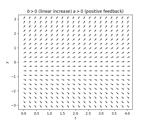
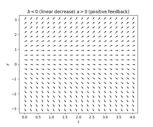
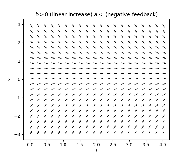
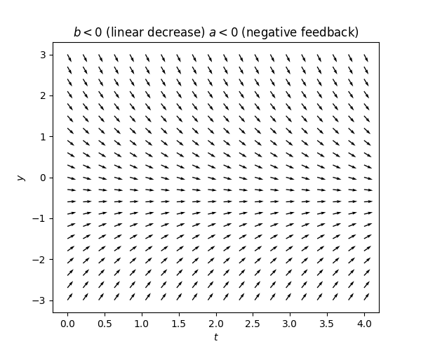
The term \(b\) represents an instantaneous absolute rate of change. Instantaneous simply because the derivative is the instantaneous rate of change of \(y(t).\) Absolute in the sense that whatever the value of \(y(t)\) is, this rate stays the same. If \(b>0\) it’s an absolute rate of increase and if \(b<0\) it’s an absolute rate of decrease.
The term \(ay(t)\) is a feedback.
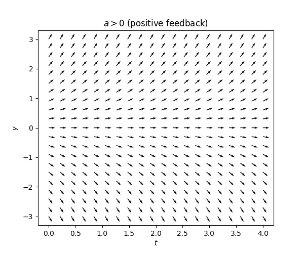
If \(a>0\) a positive feedback: the term \(ay(t)\) has the same sign as \(y(t),\) so it “tries to” make \(\dot{y}(t)\) also have this sign and thus “pushes” \(y(t)\) in the direction of increased magnitude,
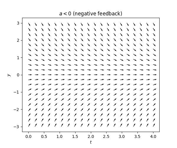
If \(a<0\) a negative feedback: the term \(ay(t)\) has the opposite sign of \(y(t),\) so it “tries to” make \(\dot{y}(t)\) also have the opposite sign and thus “pushes \(y(t)\)” in the direction of decreased magnitude.
An even more precise description of the term \(ay(t)\) is that it represents a instantaneous relative rate of range (as opposed to the absolute rate of change embodied by the term \(b\)). Relative because the amount of change is effectively given by a percentage of the current value of \(y(t),\) or in other words a proportion (namely the proportion \(a\)) of the current value of \(y(t).\)
One can see this reflected in the tangent fields of such equations:
We model the concentration of a bacterium reproducing in the blood of a patient under the following assumptions:
for each bacterium on average four child bacteria are produced per hour,
each hour one bacterium per mL of blood enters the blood stream from outside4 .Caveat: No claim is made regarding the real-world usefulness or realism of this model, it has been formulated simply to provide an instructive example which is somewhat plausible.
We refrain from modelling the effect of the immune system, or a more realistic non-constant rate of infection. Under these assumptions we let \(p(t)\) denote the concentration of bacteria per mL when \(t\) hours have passed since the patient first came into contact with the bacterium. The rate of growth of this concentration at time \(t\) is \(\dot{p}(t).\) We decompose this rate as \(\theta_{r}+\theta_{i},\) where \(\theta_{r}\) corresponds to growth due to reproduction, i.e. (1) above, and \(\theta_{i}\) corresponds to growth due to particles entering the blood from outside (“immigration” of bacteria), i.e. (2) above.
The assumption (1) can be interpreted as \(\theta_{r}=3p(t),\) since the net increase of bacteria per hour due to one bacterium is \(\text{\#child bacteria}-1=4-1=3\) .
The assumption (2) can be interpreted as \(\theta_{i}=1.\)
We call any equation of the form \[\dot{y}(t)=ay(t)+b,\quad\quad t\in I,\tag{3.10}\] for \(a,b\in\mathbb{R}\) and any interval \(I\subset\mathbb{R}\) a first order linear autonomous ODE.
We call any equation of the form \[\dot{y}(t)=ay(t)+b,\quad\quad t\in I,\tag{3.10}\] for \(a,b\in\mathbb{R}\) and any interval \(I\subset\mathbb{R}\) a first order linear autonomous ODE.
week 4: gave this equation a number, so the numbering of subsequent equations changed.
It is instructive to study solutions \(y(t)\) of ([eq:fo_lin_aut_def_eq]) via the “recentered” solutions \[x(t)=y(t)-\left(-\frac{b}{a}\right)\quad\quad t\in I,\tag{3.13}\] which represent the deviation of \(y(t)\) from the stationary solution at time \(t.\) If \(y(t)\) is a solution then \(x(t)\) satisfies \(\dot{x}(t)=\dot{y}(t)=ay(t)+b=a(y(t)+\frac{b}{a})=ax(t),\) i.e. \(x(t)\) is a solution to \[\dot{x}(t)=ax(t).\tag{3.14}\] Furthermore if \(x(t)\) is a solution to ([eq:fo_lin_aut_recentered]) then \(y(t)=x(t)+\frac{b}{a}\) is a solution of ([eq:fo_lin_aut_def_eq]) (verify this!). The equation ([eq:fo_lin_aut_recentered]) is ([eq:fo_lin_aut_def_eq]) with \(b=0,\) so we have reduced the general case with \(a\ne0,b\in\mathbb{R}\) to the case \(a\ne0,b=0.\) Note that ([eq:fo_lin_aut_recentered]) has the stationary solution \(x(t)=0,\) which makes sense since our change of variables ([eq:fo_lin_aut_cov]) has shifted all solutions down by \(-\frac{b}{a}.\)
If \(x(t)\) is a solution to ([eq:fo_lin_aut_recentered]) then \(\alpha x(t)\) is also a solution for any \(\alpha\in\mathbb{R}.\) This is not the case for the original ([eq:fo_lin_aut_def_eq]). When we study higher order linear ODEs this property will play an important role - linear ODEs that have it will be called “homogeneous”.
The tangent field for the equation ([eq:fo_lin_aut_recentered]) is simply the tangent fields from Figure Figure 3.11 shifted:
\(\text{ }\)Solution for positive feedback - \(a>0.\) From the tangent field labeled \(a>0\) in Figure Figure 3.12 we may guess that the curves traced out by the tangent is of the form \(e^{ct}\) for a positive \(c>0.\) Making the ansatz \(x(t)=e^{ct}\) and plugging into ([eq:fo_lin_aut_recentered]) we obtain that \(\dot{x}(t)=ce^{ct}=ax(t)\) for all \(t\in I\) iff \(a=c,\) and thus determine that \(x(t)=e^{at}\) is a solution. Using the property mentioned above, also \[x(t)=\alpha e^{at}\tag{3.15}\] is a solution for any \(\alpha\in\mathbb{R}.\) Going back to ([eq:ch3_fo_lin_aut-1]) this implies that \[y(t)=\alpha e^{at}-\frac{b}{a}\tag{3.16}\] is a solution for any \(\alpha\in\mathbb{R}.\) These solutions can be interpreted as functions diverging exponentially at rate \(e^{at}\) away from the stationary solution \(-\frac{b}{a}.\)
Solution for negative feedback -\(a<0.\) In this case it is instructive to highlight the negativity of the coefficient \(a\) by writing ([eq:fo_lin_aut_recentered]) in the equivalent form \[\dot{x}(t)=-|a|x(t).\tag{3.17}\]
From the tangent field labeled \(a<0\) in Figure Figure 3.12 we may guess that ([eq:ch3_fo_lin_aut_recent_a_neg]) has solutions of the form \[x(t)=e^{-ct}\text{\,for a }c>0.\tag{3.18}\] We in fact already did precisely this for ([eq:ch3_ode_grav_air_res-1]) in Section 1.3. Making the ansatz \(x(t)=e^{-ct}\) and plugging into ([eq:fo_lin_aut_recentered]) we obtain that \(\dot{x}(t)=-ce^{-ct}=-|a|x(t)\) for all \(t\in I\) iff \(|a|=c,\) and thus determine that \(x(t)=e^{-|a|t}\) is a solution. Therefore also \[x(t)=\alpha e^{-|a|t}\tag{3.19}\] is a solution for any \(\alpha\in\mathbb{R},\) and \[y(t)=\alpha e^{-|a|t}-\frac{b}{a}\tag{3.20}\] is a solution to ([eq:ch3_fo_lin_aut-1]). These solutions can be interpreted as functions converging exponentially at rate \(e^{-at}\) to the stationary solution \(-\frac{b}{a}.\)
In retrospect we see that we in fact made the same ansatz whether \(a>0,a<0,\) just with a different sign in the argument for the exponential. Whatever the sign of \(a\) we could thus simply have made the ansatz \(x(t)=e^{ct}\) for \(c\in\mathbb{R}\) and arrived at \[x(t)=\alpha e^{at},\tag{3.21}\] as a solution to ([eq:fo_lin_aut_recentered]) and \[y(t)=\alpha e^{at}-\frac{b}{a},\tag{3.22}\] as a solution to ([eq:fo_lin_aut_def_eq]) for any \(a\ne0.\)
\(\text{ }\)Ruling out other solutions. We have found the infinite family of solutions ([eq:ch3_fo_lin_aut_form_of_sol]) to ([eq:fo_lin_aut_def_eq]). Are there any other solutions? In fact, there are not! The functions ([eq:ch3_fo_lin_aut_form_of_sol]) form an exhaustive set of solutions. For the first order autonomous equations studies in this section this can be proven by an elementary argument.
(Complete solution of first order autonomous ODEs with \(a\ne0\)). Assume \(a,b\in\mathbb{R},a\ne0\) and \(I\subset\mathbb{R}\) an interval. Then a function \(y(t)\) is a solution of the ODE \[\dot{y}(t)=ay(t)+b,\quad\quad t\in I,\tag{3.23}\] iff \[y(t)=\alpha e^{at}-\frac{b}{a}\quad\forall t\in I,\text{ for some }\alpha\in\mathbb{R}.\tag{3.24}\]
Proof. \(\impliedby\) : If \(y(t)\) has the form ([eq:ch3_fo_lin_aut_uniquness_sol_form]) then \(\dot{y}(t)=a\alpha e^{at}\) and \(ay(t)+b=a(\alpha e^{at}-\frac{b}{a})+b=a\alpha e^{at}-b+b=a\alpha e^{at}=\dot{y}(t),\) so indeed \(y(t)\) solves the ODE ([eq:ch3_fo_lin_aut_uniquness_ODE_form]) .
\(\implies\): Let \(y(t)\) be any solution of ([eq:ch3_fo_lin_aut_uniquness_ODE_form]). Consider \[z(t)=e^{-at}\left(y(t)+\frac{b}{a}\right).\tag{3.25}\] Using the product rule to differentiate \(z(t)\) we obtain \[\dot{z}(t)=-ae^{-at}\left(y(t)+\frac{b}{a}\right)+e^{-at}\dot{y}(t)\text{\,for all }t\in I.\] Using that \(y(t)\) is a solution of ([eq:ch3_fo_lin_aut_uniquness_ODE_form]) by replacing \(\dot{y}(t)\) is the previous equation by the r.h.s. of ([eq:ch3_fo_lin_aut_uniquness_ODE_form]) this implies that \[\dot{z}(t)=-ae^{-at}\left(y(t)+\frac{b}{a}\right)+e^{-at}\left(ay(t)+b\right)=0\text{ for all }t\in I.\] Any differentiable function on an interval \(I\) with vanishing derivative is constant (by the fundamental theorem of calculus). Thus there is a constant \(\alpha\) such that \(z(t)=\alpha\) for all \(t\in I,\) and so \[e^{at}\left(y(t)+\frac{b}{a}\right)=\alpha\text{ for all }t\in I.\tag{3.26}\] Rearranging this implies that \(y(t)\) satisfies ([eq:ch3_fo_lin_aut_uniquness_sol_form]).
We model the concentration of a bacterium reproducing in the blood of a patient under the following assumptions:
for each bacterium on average four child bacteria are produced per hour,
each hour one bacterium per mL of blood enters the blood stream from outside4.
We refrain from modelling the effect of the immune system, or a more realistic non-constant rate of infection. Under these assumptions we let \(p(t)\) denote the concentration of bacteria per mL when \(t\) hours have passed since the patient first came into contact with the bacterium. The rate of growth of this concentration at time \(t\) is \(\dot{p}(t).\) We decompose this rate as \(\theta_{r}+\theta_{i},\) where \(\theta_{r}\) corresponds to growth due to reproduction, i.e. (1) above, and \(\theta_{i}\) corresponds to growth due to particles entering the blood from outside (“immigration” of bacteria), i.e. (2) above.
The assumption (1) can be interpreted as \(\theta_{r}=3p(t),\) since the net increase of bacteria per hour due to one bacterium is \(\text{\#child bacteria}-1=4-1=3\) .
The assumption (2) can be interpreted as \(\theta_{i}=1.\)
Thus we have arrived at the ODE model: \[\dot{p}(t)=3p(t)+1.\tag{3.11}\] The expression ([eq:ch3_bacteria]) is a first order autonomous ODE, as defined in Definition 3.10, with \(a=3\) and \(b=1\)). The “feedback” corresponding to (1), (1’), \(3p(t)\) is positive - more bacteria means faster rate growth. Indeed \(a>0.\)
We call any equation of the form \[\dot{y}(t)=ay(t)+b,\quad\quad t\in I,\tag{3.10}\] for \(a,b\in\mathbb{R}\) and any interval \(I\subset\mathbb{R}\) a first order linear autonomous ODE.
We model the concentration of a bacterium reproducing in the blood of a patient under the following assumptions:
for each bacterium on average four child bacteria are produced per hour,
each hour one bacterium per mL of blood enters the blood stream from outside4.
We refrain from modelling the effect of the immune system, or a more realistic non-constant rate of infection. Under these assumptions we let \(p(t)\) denote the concentration of bacteria per mL when \(t\) hours have passed since the patient first came into contact with the bacterium. The rate of growth of this concentration at time \(t\) is \(\dot{p}(t).\) We decompose this rate as \(\theta_{r}+\theta_{i},\) where \(\theta_{r}\) corresponds to growth due to reproduction, i.e. (1) above, and \(\theta_{i}\) corresponds to growth due to particles entering the blood from outside (“immigration” of bacteria), i.e. (2) above.
The assumption (1) can be interpreted as \(\theta_{r}=3p(t),\) since the net increase of bacteria per hour due to one bacterium is \(\text{\#child bacteria}-1=4-1=3\) .
The assumption (2) can be interpreted as \(\theta_{i}=1.\)
Thus we have arrived at the ODE model: \[\dot{p}(t)=3p(t)+1.\tag{3.11}\] The expression ([eq:ch3_bacteria]) is a first order autonomous ODE, as defined in Definition 3.10, with \(a=3\) and \(b=1\)). The “feedback” corresponding to (1), (1’), \(3p(t)\) is positive - more bacteria means faster rate growth. Indeed \(a>0.\)
The model ([eq:ch3_ode_grav_air_res-1]) of the velocity of an object subject to gravity and air resistance is an example where there is a negative feedback: for higher velocity air resistance increases. Indeed if written in the form of Definition 3.10 it has \(a=-\frac{\gamma}{m}<0.\)
We call any equation of the form \[\dot{y}(t)=ay(t)+b\quad\quad t\in I,\tag{3.28}\] for \(a,b\in\mathbb{R}\) and any interval \(I\subset\mathbb{R}\) subject to the constraint \[y(t_{0})=y_{0},\tag{3.29}\] where \(t_{0}\) is the left-endpoint of \(I\) and \(y_{0}\in\mathbb{R},\) a first order linear autonomous Initial Value Problem (IVP).
If a solution of the form ([eq:ch3_fo_lin_aut_uniquness_sol_form]) is to satisfy ([eq:fo_lin_aut_IVP_def_IVP_cond]), it must hold that \[\alpha e^{at_{0}}-\frac{b}{a}=y_{0}.\] This equation can be solved for \(\alpha\) to obtain \[\alpha=e^{-at_{0}}\left(y_{0}+\frac{b}{a}\right).\] With this value for \(\alpha\) the solution \(y(t)\) becomes \[y(t)=e^{a(t-t_{0})}\left(y_{0}+\frac{b}{a}\right)-\frac{b}{a}.\tag{3.30}\] The function ([eq:ch3_fo_aut_IVP_sol]) is a solution to the ODE ([eq:fo_lin_aut_def_eq]) subject to the constraint ([eq:ch3_fo_lin_aut_IVP_cond]). It follows by the previous lemma, and the fact that \(\alpha\) above is unique, that this is the unique solution.
Assume \(a,b\in\mathbb{R},\) \(a\ne0,\) \(I\subset\mathbb{R}\) an interval \(t_{*}\in I\) and \(y_{0}\in\mathbb{R}.\) Then the ODE \[\dot{y}(t)=ay(t)+b\quad t\in I,\tag{3.31}\] subject to the constraint \[y(t_{*})=y_{0},\tag{3.32}\] has the unique solution \[y(t)=\left(y_{0}+\frac{b}{a}\right)e^{a(t-t_{*})}-\frac{b}{a}\quad\forall t\in I.\tag{3.33}\]
(Complete solution of first order autonomous ODEs with \(a\ne0\)). Assume \(a,b\in\mathbb{R},a\ne0\) and \(I\subset\mathbb{R}\) an interval. Then a function \(y(t)\) is a solution of the ODE \[\dot{y}(t)=ay(t)+b,\quad\quad t\in I,\tag{3.23}\] iff \[y(t)=\alpha e^{at}-\frac{b}{a}\quad\forall t\in I,\text{ for some }\alpha\in\mathbb{R}.\tag{3.24}\]
(Complete solution of first order autonomous ODEs with \(a\ne0\)). Assume \(a,b\in\mathbb{R},a\ne0\) and \(I\subset\mathbb{R}\) an interval. Then a function \(y(t)\) is a solution of the ODE \[\dot{y}(t)=ay(t)+b,\quad\quad t\in I,\tag{3.23}\] iff \[y(t)=\alpha e^{at}-\frac{b}{a}\quad\forall t\in I,\text{ for some }\alpha\in\mathbb{R}.\tag{3.24}\]
a) In exercise \(1.\) on exercise sheet \(2\) you will practice solving this kind of ODE.
b) If you are solving a given concrete first order linear autonomous ODE, it is recommended that you make the ansatz \(y(t)=Ae^{Bt}+C\) and then solve for \(A,B,C\) that satisfy the ODE and any constraints you may want to satisfy, rather than memorizing and using the explicit formula ([eq:ch3_fo_lin_aut_IVP_uniq_sol]). The implicit general form \(y(t)=Ae^{Bt}+C\) is easier to remember, the computation using it will be less error prone, and if you ever need the general explicit formula ([eq:ch3_fo_lin_aut_IVP_uniq_sol]) you easily rederive it from the former implicit form.
(Complete solution of first order autonomous ODEs with \(a\ne0\)). Assume \(a,b\in\mathbb{R},a\ne0\) and \(I\subset\mathbb{R}\) an interval. Then a function \(y(t)\) is a solution of the ODE \[\dot{y}(t)=ay(t)+b,\quad\quad t\in I,\tag{3.23}\] iff \[y(t)=\alpha e^{at}-\frac{b}{a}\quad\forall t\in I,\text{ for some }\alpha\in\mathbb{R}.\tag{3.24}\]
\(\text{ }\)No feedback - special case \(a=0\) The above results dealt with the main case of the ODE ([eq:fo_lin_aut_def_eq]), which is \(a\ne0.\) For completeness we finish by handling the case \(a=0,\) for which the solutions behave differently - they are linear functions.
(Solution of first order autonomous ODEs with \(a=0\)). Assume \(b\in\mathbb{R}\) and \(I\subset\mathbb{R}\) an interval. Then a function \(y\) is a solution of the ODE \[\dot{y}(t)+b=0,\quad\quad t\in I,\] iff \[y(t)=\alpha-bt\quad\forall t\in I,\text{ for some }\alpha\in\mathbb{R}.\]
Proof. Exercise (exercise 2 on exercise sheet 2).
3.3 Explicit and implicit ODEs
If \(k\ge1\) and \({G:\mathbb{R}^{k+2}\to\mathbb{R}}\) and \(I\subset\mathbb{R}\) is an interval we call the expression \[G(t,f^{(k)}(t),f^{(k-1)}(t),\ldots,f^{'}(t),f(t))=0\quad t\in I,\tag{2.7}\] an Ordinary Differential Equation of order \(k.\) We call any \(k\)-times differential function \(h:I\to\mathbb{R}\) such that \[G(t,h^{(k)}(t),h^{(k-1)}(t),\ldots,h^{'}(t),h(t))=0\quad\forall t\in I,\] solution to the ODE ([eqn:ODE_def]) on the interval \(I.\)
week 2 v2: added formal definition of domain of \(H\)
The implicit form ([eq:ch3_implicit_eq]) is more general: every explicit ODE of the form ([eq:ch3_explicit_eq]) is also of the form ([eq:ch3_implicit_eq]) with \(G(t,y_{k},\ldots,y_{0})=y_{k}-H(t,y_{k-1},\ldots,y_{0}).\) Sometimes an ODE written in the implicit form ([eq:ch3_implicit_eq]) can conversely easily be written in the explicit form ([eq:ch3_explicit_eq]). This was the case in the previous section where the ODEs \[\alpha\dot{y}(t)+\beta y(t)+\gamma=0,\quad\quad t\in I,\] (see ([eq:ch3_fo_lin_aut-1]); this is an implicit relation) with constant coefficients and \(\alpha\ne0\) were seen to be equivalent to an ODE of the form \[\dot{y}(t)=ay+b,\quad\quad t\in I,\] (see ([eq:fo_lin_aut_def_eq]); this is explicit). Another such example is the implicit ODE \[(1+t^{2})\ddot{y}(t)+\dot{y}(t)y(t)=5,\quad\quad t\in\mathbb{R},\tag{3.37}\] corresponding to ([eq:ch3_implicit_eq]) with \(k=2\) and \(G(t,y_{2},y_{1},y_{0})=(1+t)^{2}y_{2}+y_{1}y_{0}-5.\) Since the coefficient \(1+t^{2}\)of \(\ddot{y}(t)\) is everywhere positive the relation ([eq:ch3_non_lin_implicit_ex]) can be solved for \(\ddot{y}(t)\) to obtain \[\ddot{y}(t)+\frac{\dot{y}(t)y(t)-5}{1+t^{2}}=0,\quad\quad t\in\mathbb{R},\] which is of the explicit form ([eq:ch3_explicit_eq]) with \(H(t,y_{1},y_{0})=-\frac{y_{1}y_{0}-5}{1+t^{2}}.\)
But for instance the ODE written implicitly as \[t\ddot{y}(t)+\dot{y}(t)y(t)=5,\quad\quad t\in[-1,1],\] can not be directly written explicitly on the interval \([-1,1],\) since we can not divide through by the coefficient \(t\) for \(t=0.\) Another such example is the implicitly written ODE \[(\dot{y}(t))^{2}-y(t)^{2}-1=0,\quad\quad t\in[0,\infty).\tag{3.38}\] The condition ([eq:ch3_non_lim_implicit_ex_not_explicit]) is equivalent to \[\dot{y}(t)=\pm\sqrt{1+y(t)^{2}},\quad\quad t\in[0,\infty),\] which is not of the form ([eq:ch3_explicit_eq]) for a single function \(H,\) because of the \(\pm\) coming from the two possible square roots.
A first order explicit ODE is simply the case \(k=1\) of ([eq:ch3_explicit_eq]).
We call any ODE of the form \[\dot{x}(t)=H(t,x(t)),\quad\quad t\in I,\tag{3.40}\] for a function \(H:\mathbb{R}^{2}\to\mathbb{R}\) and interval \(I\subset\mathbb{R}\) an explicit first order ODE.
We call any ODE of the form \[\dot{x}(t)=H(x(t)),\quad\quad t\in I,\tag{3.41}\] for a function \(H:\mathbb{R}\to\mathbb{R}\) and interval \(I\subset\mathbb{R}\) an explicit first order autonomous ODE.
We call ([eq:def_ch3_fo_explicit]) or ([eq:def_ch3_fo_aut]) together with the constraint \[x(t_{0})=x_{0},\tag{3.42}\] where \(t_{0}\) is the left-endpoint of \(I\) and \(x_{0}\in\mathbb{R}\) an explicit first order Initial Value Problem (IVP).
Compare ([eq:def_ch3_fo_explicit]) to ([eqn:ODE_def]), ([eq:def_ch3_fo_aut]) to ([eq:ODE_def-1]) and ([eq:def_ch3_fo_explicit_IVP]) to ([eq:fo_lin_aut_IVP_def_IVP_cond]). This form of ODE has already been mentioned in passing in ([eq:ch3_tf_first_order_aut_explicit]) and ([eq:ch3_preview_fo_general_IVP]). In the next few sections we will study explicit first order ODEs like ([eq:def_ch3_fo_explicit]). Before the end of the chapter will consider the implicit first order linear equations \(\alpha(t)\dot{y}(t)+\beta(t)y(t)+\gamma(t)=0.\)
3.4 Interlude - Leibniz rule for differentiating under the integral sign
When solving non-autonomous first order linear equations in the next section we will need to compute derivatives of the form \[\frac{d}{dt}\int_{s}^{t}f(r,t)dr.\] The classical formula for these is known as Leibniz rule. Recall that the fundamental theorem of calculus addresses the case when \(f\) does not depend on \(t,\) and states that \[\frac{d}{dt}\int_{s}^{t}f(r)dr=f(t)\tag{3.43}\] for any Lebesgue integrable function \(f.\) Leibniz rule is the following.
If \(I\subset\mathbb{R}\) is an open interval and \(f:I^{2}\to\mathbb{R}\) is such that \(f(r,t)\) is continuous in \(I^{2},\) and the partial derivative \(\partial_{t}f(r,t)\) exists and is continuous in \(I^{2},\) then the derivative \(\frac{d}{dt}\int_{s}^{t}f(r,t)dr\) is well-defined for all \(s,t\in I,s\le t,\) and \[\frac{d}{dt}\int_{s}^{t}f(r,t)dr=f(t,t)+\int_{s}^{t}\partial_{t}f(r,t)dr.\]
Heuristically this formula may be derived by using the Taylor expansion \[f(r,t+\varepsilon)=f(r,t)+\varepsilon\partial_{t}f(r,t)+O(\varepsilon^{2}),\] and using the definition of the derivative as the limit \[\lim_{\varepsilon\to0}\varepsilon^{-1}\left(\int_{s}^{t+\varepsilon}f(r,t+\varepsilon)dr-\int_{s}^{t}f(r,t)dr\right),\] together with the fundamental theorem of calculus ([eq:ftoc]).
3.5 Explicit first order linear non-autonomous equations
We call any equation of the form \[\dot{y}(t)=ay(t)+b,\quad\quad t\in I,\tag{3.10}\] for \(a,b\in\mathbb{R}\) and any interval \(I\subset\mathbb{R}\) a first order linear autonomous ODE.
We call any ODE of the form \[\dot{x}(t)=H(t,x(t)),\quad\quad t\in I,\tag{3.40}\] for a function \(H:\mathbb{R}^{2}\to\mathbb{R}\) and interval \(I\subset\mathbb{R}\) an explicit first order ODE.
We call any ODE of the form \[\dot{x}(t)=H(x(t)),\quad\quad t\in I,\tag{3.41}\] for a function \(H:\mathbb{R}\to\mathbb{R}\) and interval \(I\subset\mathbb{R}\) an explicit first order autonomous ODE.
We call ([eq:def_ch3_fo_explicit]) or ([eq:def_ch3_fo_aut]) together with the constraint \[x(t_{0})=x_{0},\tag{3.42}\] where \(t_{0}\) is the left-endpoint of \(I\) and \(x_{0}\in\mathbb{R}\) an explicit first order Initial Value Problem (IVP).
We call any equation of the form \[\dot{y}(t)=a(t)y(t)+b(t),\quad\quad t\in I,\tag{3.45}\] for any interval \(I\subset\mathbb{R}\) and functions \(a,b:I\to\mathbb{R}\) an explicit first order linear ODE.
We actually find explicit formulas for the solutions, which are somewhat related to those of Section 3.2 for the autonomous case, albeit somewhat more complex.
We call any equation of the form \[\dot{y}(t)=a(t)y(t)+b(t),\quad\quad t\in I,\tag{3.45}\] for any interval \(I\subset\mathbb{R}\) and functions \(a,b:I\to\mathbb{R}\) an explicit first order linear ODE.
\(\text{ }\)Interpretation. One can interpret the ODE ([eq:fo_lin_def_eq]) as follows.
The term \(b(t)\): Recall from Section 3.2 that in the autonomous case \(\dot{y}(t)=ay(t)+b\) the term \(b\) can be thought of as an instantaneous absolute rate of change. In the autonomous case this rate is constant. The same interpretation works in the non-autonomous case - the rate \(b(t)\) simply varies with the independent variable \(t.\)
The term \(a(t)y(t)\): Recall that in the autonomous case the term \(ay(t)\) can be thought of as positive or negative feedback depending on the sign of \(a,\) and as an instantaneous relative rate of change. In the autonomous case this rate is constant, but in the non-autonomous case the same interpretation works - the instantaneous relative change simply changes with \(t,\) and can switch between acting as a positive or negative feedback depending on the sign of \(a(t).\)
\(\text{ }\)Solution when \(b(t)=0\) We consider first the case \(b(t)=0\) of ([eq:fo_lin_def_eq]), namely \[\dot{x}(t)=a(t)x(t),\quad\quad t\in I.\tag{3.47}\] This is ([eq:fo_lin_aut_recentered]) with a non-constant coefficient \(a(t).\) As for ([eq:fo_lin_aut_recentered]), if \(x(t)\) is a solution to ([eq:ch3_fo_lin_b_zero]) then so is \(t\to\alpha x(t)\) for any \(\alpha\in\mathbb{R}.\)
Assume \(a,b\in\mathbb{R},\) \(a\ne0,\) \(I\subset\mathbb{R}\) an interval \(t_{*}\in I\) and \(y_{0}\in\mathbb{R}.\) Then the ODE \[\dot{y}(t)=ay(t)+b\quad t\in I,\tag{3.31}\] subject to the constraint \[y(t_{*})=y_{0},\tag{3.32}\] has the unique solution \[y(t)=\left(y_{0}+\frac{b}{a}\right)e^{a(t-t_{*})}-\frac{b}{a}\quad\forall t\in I.\tag{3.33}\]
If \(a(t)\) is constant it reduces to \(x(t)=e^{ta}x(0)\) which we know is the solution in this case (by Proposition 3.15 Proposition 3.15 • Unique solution of first order linear autonomous ODEs with constraint ➔).Assume \(a,b\in\mathbb{R},\) \(a\ne0,\) \(I\subset\mathbb{R}\) an interval \(t_{*}\in I\) and \(y_{0}\in\mathbb{R}.\) Then the ODE \[\dot{y}(t)=ay(t)+b\quad t\in I,\tag{3.31}\] subject to the constraint \[y(t_{*})=y_{0},\tag{3.32}\] has the unique solution \[y(t)=\left(y_{0}+\frac{b}{a}\right)e^{a(t-t_{*})}-\frac{b}{a}\quad\forall t\in I.\tag{3.33}\]
In terms of the above interpretation, the instantaneous relative rate of change is \(a(t)\) and over the time interval \([0,t]\) is accumulates via the integral \(\int_{0}^{t}a(s)ds.\)
The second point makes sense for any (integrable) \(a(t),\) piece-wise constant or not. Thus it makes sense to try ([eq:ch3_fo_lin_b_zero_ansatz_interval_0_1]) as an ansatz for a solution of ([eq:ch3_fo_lin_b_zero]) for general \(a(t).\)
Let \(I\subset\mathbb{R}\) be an interval and let \(a,b:I\to\mathbb{R}\) be continuous and Lebesgue integrable on \(I.\)
A function \(y:I\to\mathbb{R}\) is a solution to the ODE \[\dot{y}(t)=a(t)y(t)+b(t),\quad\quad t\in I,\tag{3.60}\] iff \[y(t)=\alpha e^{\int_{t_{0}}^{t}a(s)ds}+\int_{t_{0}}^{t}e^{\int_{r}^{t}a(s)ds}b(r)dr,\quad\quad t\in I,\tag{3.61}\] for some \(\alpha\in\mathbb{R}.\)
\(\text{ }\)Heuristically deriving ansatz for \(b(t)\ne0\) Recall that we interpret \(b(t)\) as an instantaneous absolute rate of change. Over a small time interval \([t,t+\varepsilon)\) the cumulative absolute change can be thought of as approximately \(\varepsilon b(t).\) Heuristically, things become simpler if we imagine instead that the whole absolute change of magnitude \(\sim\varepsilon b(t)\) happens in one instantaneous jump at the start of the time interval, at time \(t.\) For instance, we can imagine jumps of size \(\varepsilon b(t_{n})\) at times \(t_{0}+n\varepsilon.\) In this case a solution between the jump times, in the open interval \((t_{n},t_{n+1})\) would evolve as ([eq:ch3_fo_lin_b_zero]), without a \(b(t)\) term. Then at time \(t=t_{n+1}\) one would have a sudden increase from \(y(t_{n+1}^{-})\) (the left limit as \(t=t_{n+1})\) to \(y(t_{n+1}^{+})=y(t_{n+1}^{-})+\varepsilon b(t_{n+1})\) (the right limit at \(t=t_{n+1}\)), and then in the time interval \((t_{n+1},t_{n+2})\) the solution would evolve as ([eq:ch3_fo_lin_b_zero]) again.
week 2 v2: added interval explicitly for clarity
Continuing in the same manner for \(n-1,n-2,\ldots,0\) and multiplying out would give \[y(t)=y(t_{0}^{-})e^{\int_{t_{0}}^{t}a(s)ds}+\varepsilon\sum_{k=0}^{n}b(t_{k})e^{\int_{t_{k}}^{t}a(s)ds},\quad\quad t\in(t_{n+1},t_{n+2}).\]
Here the interpretation is that at time \(t_{k}\) the level of \(y(t)\) jumps by \(\varepsilon b(t_{k}),\) and the size of the jump then evolves as the ODE \(\dot{x}(t)=a(t)x(t)\) until the time \(t,\) giving a final contribution of \(\varepsilon b(t_{k})e^{\int_{t_{k}}^{t}a(s)ds}.\) The sum in this expression can be thought of as a Riemann sum which approximates the integral \(\int_{0}^{t}b(r)e^{\int_{r}^{t}a(s)ds}dr,\) which is a well-defined quantity also in our original setting of function \(b(t)\) representing an instantaneous absolute rate of increase without any “jumping”. This leads us to the ansatz \[y(t)=y(t_{0})e^{\int_{t_{0}}^{t}a(s)ds}+\int_{t_{0}}^{t}b(r)e^{\int_{r}^{t}a(s)ds}dr,\quad\quad t\in I,\tag{3.55}\] with the interpret that at time \(r\) an “infinitesimal amount” \(b(r)\) is added to \(y(t),\) and this contribution then evolves in the interval \([r,t]\) as the ODE \(\dot{x}(t)=a(t)x(t).\)
Assume \(a,b\in\mathbb{R},\) \(a\ne0,\) \(I\subset\mathbb{R}\) an interval \(t_{*}\in I\) and \(y_{0}\in\mathbb{R}.\) Then the ODE \[\dot{y}(t)=ay(t)+b\quad t\in I,\tag{3.31}\] subject to the constraint \[y(t_{*})=y_{0},\tag{3.32}\] has the unique solution \[y(t)=\left(y_{0}+\frac{b}{a}\right)e^{a(t-t_{*})}-\frac{b}{a}\quad\forall t\in I.\tag{3.33}\]
Let \(I\subset\mathbb{R}\) be an interval and let \(a,b:I\to\mathbb{R}\) be continuous and Lebesgue integrable on \(I.\)
A function \(y:I\to\mathbb{R}\) is a solution to the ODE \[\dot{y}(t)=a(t)y(t)+b(t),\quad\quad t\in I,\tag{3.60}\] iff \[y(t)=\alpha e^{\int_{t_{0}}^{t}a(s)ds}+\int_{t_{0}}^{t}e^{\int_{r}^{t}a(s)ds}b(r)dr,\quad\quad t\in I,\tag{3.61}\] for some \(\alpha\in\mathbb{R}.\)
If \(I\subset\mathbb{R}\) is an open interval and \(f:I^{2}\to\mathbb{R}\) is such that \(f(r,t)\) is continuous in \(I^{2},\) and the partial derivative \(\partial_{t}f(r,t)\) exists and is continuous in \(I^{2},\) then the derivative \(\frac{d}{dt}\int_{s}^{t}f(r,t)dr\) is well-defined for all \(s,t\in I,s\le t,\) and \[\frac{d}{dt}\int_{s}^{t}f(r,t)dr=f(t,t)+\int_{s}^{t}\partial_{t}f(r,t)dr.\]
Let \(I\subset\mathbb{R}\) be an interval and let \(a,b:I\to\mathbb{R}\) be continuous and Lebesgue integrable on \(I.\)
A function \(y:I\to\mathbb{R}\) is a solution to the ODE \[\dot{y}(t)=a(t)y(t)+b(t),\quad\quad t\in I,\tag{3.60}\] iff \[y(t)=\alpha e^{\int_{t_{0}}^{t}a(s)ds}+\int_{t_{0}}^{t}e^{\int_{r}^{t}a(s)ds}b(r)dr,\quad\quad t\in I,\tag{3.61}\] for some \(\alpha\in\mathbb{R}.\)
(Complete solution of first order autonomous ODEs with \(a\ne0\)). Assume \(a,b\in\mathbb{R},a\ne0\) and \(I\subset\mathbb{R}\) an interval. Then a function \(y(t)\) is a solution of the ODE \[\dot{y}(t)=ay(t)+b,\quad\quad t\in I,\tag{3.23}\] iff \[y(t)=\alpha e^{at}-\frac{b}{a}\quad\forall t\in I,\text{ for some }\alpha\in\mathbb{R}.\tag{3.24}\]
The fundamental theorem of calculus implies the following.
If \(a:I\to\mathbb{R}\) is continuous and Lebesgue integrable then \(t\to e^{\int_{r}^{t}a(s)ds}\) is continuous and differentiable in \(I,\) and \[\frac{d}{dt}e^{\int_{r}^{t}a(s)ds}=a(t)e^{\int_{r}^{t}a(s)ds},\quad\quad t\in I.\]
Leibniz’s rule implies the following.
Let \(I\subset\mathbb{R}\) be an interval and let \(a,b:I\to\mathbb{R}\) be continuous and Lebesgue integrable on \(I.\) Then \[t\to\int_{t_{0}}^{t}e^{\int_{r}^{t}a(s)ds}b(r)dr,\quad\quad t\in I,\] is well-defined and differentiable, and \[\frac{d}{dt}\int_{t_{0}}^{t}e^{\int_{r}^{t}a(s)ds}b(r)dr=b(t)+a(t)\int_{t_{0}}^{t}e^{\int_{r}^{t}a(s)ds}b(r)dr.\tag{3.58}\]
If \(a:I\to\mathbb{R}\) is continuous and Lebesgue integrable then \(t\to e^{\int_{r}^{t}a(s)ds}\) is continuous and differentiable in \(I,\) and \[\frac{d}{dt}e^{\int_{r}^{t}a(s)ds}=a(t)e^{\int_{r}^{t}a(s)ds},\quad\quad t\in I.\]
If \(I\subset\mathbb{R}\) is an open interval and \(f:I^{2}\to\mathbb{R}\) is such that \(f(r,t)\) is continuous in \(I^{2},\) and the partial derivative \(\partial_{t}f(r,t)\) exists and is continuous in \(I^{2},\) then the derivative \(\frac{d}{dt}\int_{s}^{t}f(r,t)dr\) is well-defined for all \(s,t\in I,s\le t,\) and \[\frac{d}{dt}\int_{s}^{t}f(r,t)dr=f(t,t)+\int_{s}^{t}\partial_{t}f(r,t)dr.\]
We are now ready to prove to characterize all solutions to the first order linear ODE ([eq:fo_lin_def_eq]).
Let \(I\subset\mathbb{R}\) be an interval and let \(a,b:I\to\mathbb{R}\) be continuous and Lebesgue integrable on \(I.\)
A function \(y:I\to\mathbb{R}\) is a solution to the ODE \[\dot{y}(t)=a(t)y(t)+b(t),\quad\quad t\in I,\tag{3.60}\] iff \[y(t)=\alpha e^{\int_{t_{0}}^{t}a(s)ds}+\int_{t_{0}}^{t}e^{\int_{r}^{t}a(s)ds}b(r)dr,\quad\quad t\in I,\tag{3.61}\] for some \(\alpha\in\mathbb{R}.\)
If \(a:I\to\mathbb{R}\) is continuous and Lebesgue integrable then \(t\to e^{\int_{r}^{t}a(s)ds}\) is continuous and differentiable in \(I,\) and \[\frac{d}{dt}e^{\int_{r}^{t}a(s)ds}=a(t)e^{\int_{r}^{t}a(s)ds},\quad\quad t\in I.\]
Let \(I\subset\mathbb{R}\) be an interval and let \(a,b:I\to\mathbb{R}\) be continuous and Lebesgue integrable on \(I.\) Then \[t\to\int_{t_{0}}^{t}e^{\int_{r}^{t}a(s)ds}b(r)dr,\quad\quad t\in I,\] is well-defined and differentiable, and \[\frac{d}{dt}\int_{t_{0}}^{t}e^{\int_{r}^{t}a(s)ds}b(r)dr=b(t)+a(t)\int_{t_{0}}^{t}e^{\int_{r}^{t}a(s)ds}b(r)dr.\tag{3.58}\]
If \(a:I\to\mathbb{R}\) is continuous and Lebesgue integrable then \(t\to e^{\int_{r}^{t}a(s)ds}\) is continuous and differentiable in \(I,\) and \[\frac{d}{dt}e^{\int_{r}^{t}a(s)ds}=a(t)e^{\int_{r}^{t}a(s)ds},\quad\quad t\in I.\]
Let \(I\subset\mathbb{R}\) be an interval and let \(a,b:I\to\mathbb{R}\) be continuous and Lebesgue integrable on \(I.\) Then \[t\to\int_{t_{0}}^{t}e^{\int_{r}^{t}a(s)ds}b(r)dr,\quad\quad t\in I,\] is well-defined and differentiable, and \[\frac{d}{dt}\int_{t_{0}}^{t}e^{\int_{r}^{t}a(s)ds}b(r)dr=b(t)+a(t)\int_{t_{0}}^{t}e^{\int_{r}^{t}a(s)ds}b(r)dr.\tag{3.58}\]
Also similarly to the autonomous case, we get uniqueness of the solution to IVPs.
Let \(I\subset\mathbb{R}\) be an interval and let \(a,b:I\to\mathbb{R}\) be continuous and Lebesgue integrable on \(I.\) A function \(y:I\to\mathbb{R}\) is a solution to the IVP \[\dot{y}(t)=a(t)y(t)+b(t),\quad\quad t\in I,\quad\quad y(t_{0})=y_{0},\] iff \[y(t)=y_{0}e^{\int_{t_{0}}^{t}a(s)ds}+\int_{t_{0}}^{t}e^{\int_{r}^{t}a(s)ds}b(r)dr,\quad\quad t\in I.\]
Assume \(a,b\in\mathbb{R},\) \(a\ne0,\) \(I\subset\mathbb{R}\) an interval \(t_{*}\in I\) and \(y_{0}\in\mathbb{R}.\) Then the ODE \[\dot{y}(t)=ay(t)+b\quad t\in I,\tag{3.31}\] subject to the constraint \[y(t_{*})=y_{0},\tag{3.32}\] has the unique solution \[y(t)=\left(y_{0}+\frac{b}{a}\right)e^{a(t-t_{*})}-\frac{b}{a}\quad\forall t\in I.\tag{3.33}\]
Assume \(a,b\in\mathbb{R},\) \(a\ne0,\) \(I\subset\mathbb{R}\) an interval \(t_{*}\in I\) and \(y_{0}\in\mathbb{R}.\) Then the ODE \[\dot{y}(t)=ay(t)+b\quad t\in I,\tag{3.31}\] subject to the constraint \[y(t_{*})=y_{0},\tag{3.32}\] has the unique solution \[y(t)=\left(y_{0}+\frac{b}{a}\right)e^{a(t-t_{*})}-\frac{b}{a}\quad\forall t\in I.\tag{3.33}\]
Some of the problems in exercise 3, 4, 5 on exercise sheet 2 can be solved with the methods of this section.
3.6 Separable first order equations
Separable first order equations are an important class of ODE that admit quite explicit solutions even beyond linear case of the last section. In this context it is convenient to use Leibniz’s notation \(\frac{dy}{dx}\) for the derivative.
\(\text{ }\)Trivially separable ODE. Consider the ODE \[\frac{dy}{dx}=x^{3},\quad\quad x\in\mathbb{R},\tag{3.65}\] for an unknown function \(y.\) This is a trivial ODE, because the r.h.s. does not depend on \(y,\) only on the independent variable \(x.\) It is thus a simple integration problem: integrating both sides against \(x\) we obtain using the fundamental theorem of calculus for the l.h.s. that \[\int_{a}^{b}\frac{dy}{dx}dx=y(b)-y(a),\text{\,for all }a,b\in\mathbb{R},\tag{3.66}\] and for the r.h.s. that \[\int_{a}^{b}x^{3}dx=\frac{x^{4}}{4}|_{a}^{b}=\frac{b^{4}}{4}-\frac{a^{4}}{4},\text{\,for all }a,b\in\mathbb{R}.\tag{3.67}\] Thus any solution to ([eq:ch3_sep_trivial_example]) must satisfy \[y(b)-y(a)=\frac{b^{4}}{4}-\frac{a^{4}}{4}\text{\,for all }a,b\in\mathbb{R}.\] This implies that \[y(x)=c+\frac{x^{4}}{4},\tag{3.68}\] for the constant \(c=y(a)-\frac{a^{4}}{4}.\) It is easy to check that for any \(c\in\mathbb{R},\) the function ([eq:ch3_fo_sep_just_integration]) indeed satisfies ([eq:ch3_sep_trivial_example]). One could more quickly arrive at ([eq:ch3_fo_sep_just_integration]) by using the indefinite integrals \(\int\frac{dy}{dx}dx=y(x)+c'\) and \(\int xdx=\frac{x^{2}}{2}+c'',\) where arbitrary constants appear because indefinite integrals are only defined up to additive constant.
\(\text{ }\) Non-trivial separable ODE. Consider now the ODE \[\frac{dy}{dx}=6y^{2}x,\quad\quad x\in\mathbb{R}.\tag{3.69}\] Here is a very powerful heuristic trick to guess solutions of such an equation. Pretend that \(\frac{dy}{dx}\) is a fraction of two “infinitesimal variables” \(dx\) and \(dy,\) which it properly speaking is not: it is the derivative of \(y\) with respect to \(x,\) and \(dx\) and \(dy\) have no proper meaning if they appear by themselves, outside an integral like in ([eq:ch3_sep_trivial_rhs]) and ([eq:ch3_sep_trivial_lhs]) (in the integral the notation simply indicates which variable is integrated over, it does not represent a variable itself). Nevertheless, “squinting” and treating \(dy\) and \(dx\) as if they were variables we can multiply both sides of the equation by \(dx\) and cancel \(dx\) on the l.h.s. to obtain \["dy=6y^{2}xdx".\tag{3.70}\] The quotation marks indicate that this not a proper mathematically well-defined equation, only a heuristic way to rewrite the ([eq:ch3_sep_first_example]) . We can then divide through by \(y^{2},\) to obtain \["\frac{dy}{y^{2}}=6xdx".\tag{3.71}\] Now let us apply an indefinite integral to both sides \["\int\frac{dy}{y^{2}}=6\int xdx+c".\tag{3.72}\] The constant \(c\) appears since an indefinite integral is only defined up to additive constant.This is a well-defined expression: both sides are integrals with proper rigorous mathematical meaning! But the quotation marks remain because of the non-rigorous heuristic derivation that led to ([eq:ch3_sep_first_example_res]). We can compute both integrals in ([eq:ch3_sep_first_example_res]): \[\int\frac{dy}{y^{2}}=-\frac{1}{y}\text{ and }\int xdx=\frac{x^{2}}{2}.\tag{3.73}\] Combing these with ([eq:ch3_sep_first_example_res]) gives \["-\frac{1}{y}=3x^{2}+c".\tag{3.74}\] Solving for \(y\) gives \["y=\frac{1}{c-3x^{2}}".\tag{3.75}\]
\(\text{ }\) Trying ansatz. We can now consider this expression an ansatz for a solution of ([eq:ch3_sep_first_example]), i.e. we assume that \[y(x)=\frac{1}{c-3x^{2}},\tag{3.76}\] for some \(c\in\mathbb{R}.\) For this \(y(x)\) we have \[6y^{2}x=6\left(\frac{1}{c-3x^{2}}\right)^{2}x=\frac{6x}{(c-3x^{2})^{2}}.\] Furthermore using the chain rule we obtain \[\frac{dy}{dx}=-\frac{\frac{d}{dx}\left(c-3x^{2}\right)}{\left(c-3x^{2}\right)^{2}}=\frac{6x}{(c-3x^{2})^{2}}-.\] Thus indeed this \(y(x)\) satisfies the ODE ([eq:ch3_sep_first_example])! At least, on any interval \(I\) where \(y(x)\) as in ([eq:ch3_fo_sep_first_example_ansatz]) is well-defined and differentiable. This interval depends on \(c.\) If \(c<0\) then ([eq:ch3_fo_sep_first_example_ansatz]) is well-defined on the whole real line so one can take \(I=\mathbb{R}.\) If \(c\ge0\) then ([eq:ch3_fo_sep_first_example_ansatz]) is well-defined except when \(c=3x^{2},\) i.e. for \(x=\pm\sqrt{\frac{c}{3}}.\) Thus ([eq:ch3_fo_sep_first_example_ansatz]) is well-defined and differentiable on the three intervals \((-\infty,-\sqrt{\frac{c}{3}}),(-\sqrt{\frac{c}{3}},\sqrt{\frac{c}{3}})\) and \((\sqrt{\frac{c}{3}},\infty),\) and solves the ODE ([eq:ch3_sep_first_example]) on these intervals.
\(\text{ }\) Separable IVP. We can also use this family of solutions to derive solutions to IVPs such as \[\frac{dy}{dx}=6y^{2}x,\quad\quad y(0)=1.\tag{3.77}\] We seek a \(c\) such that \[\frac{1}{c-3x^{2}}=1\] when \(x=0,\) which simply means that \(c=1.\) Thus \[y(x)=\frac{1}{1-3x^{2}},\tag{3.78}\] is a solution to the IVP ([eq:ch3_fo_first_example_IVP]). However, we must once again be careful about the interval where the solution is defined and satisfies the ODE: in this case it is \([0,\frac{1}{\sqrt{3}}).\) As \(t\uparrow\frac{1}{\sqrt{3}}\) the solution ([eq:ch3_fo_first_example_IVP_sol]) diverges to \(\infty,\) and therefore is not defined for \(t=\frac{1}{\sqrt{3}}.\)
In fact for any \(y_{0}\in\mathbb{R}\) the IVP \[\frac{dy}{dx}=6y^{2}x,\quad\quad y(0)=y_{0},\] has the solution \[y(x)=\frac{1}{y_{0}-3x^{2}}\text{ on the interval }I=[0,\frac{y_{0}}{\sqrt{3}}),\] with the exception of \(y_{0}=0\): there is no solution in the family ([eq:ch3_fo_sep_first_example_ansatz]) which solves the IVP with \(y_{0}=0.\)
\(\text{ }\) Summary. Miraculously, the seemingly nonsense computations ([eq:ch3_fo_first_example_1])-([eq:ch3_fo_first_example_res_3]) led to a whole family of actual bona-fide solutions to the ODE ([eq:ch3_sep_first_example]). The crucial part of the nonsense computation was the separation that is expressed in ([eq:ch3_fo_first_example_1]): \(y\) only appears on the l.h.s. and \(x\) only appears on the r.h.s. Whenever an ODE can be written in a factored form \[\frac{dy}{dx}=\frac{p(x)}{q(y)}\tag{3.79}\] one can carry out an analogous heuristic computation after “splitting” \(\frac{dy}{dx}.\) One obtains \["q(y)dy=p(x)dx",\] and if both sides can be integrated one obtains an ansatz for a solution that can then be verified rigorously.
\(\text{ }\) Other examples. Let us try this procedure for linear first order ODEs.
(Complete solution of first order autonomous ODEs with \(a\ne0\)). Assume \(a,b\in\mathbb{R},a\ne0\) and \(I\subset\mathbb{R}\) an interval. Then a function \(y(t)\) is a solution of the ODE \[\dot{y}(t)=ay(t)+b,\quad\quad t\in I,\tag{3.23}\] iff \[y(t)=\alpha e^{at}-\frac{b}{a}\quad\forall t\in I,\text{ for some }\alpha\in\mathbb{R}.\tag{3.24}\]
Let \(I\subset\mathbb{R}\) be an interval and let \(a,b:I\to\mathbb{R}\) be continuous and Lebesgue integrable on \(I.\) A function \(y:I\to\mathbb{R}\) is a solution to the IVP \[\dot{y}(t)=a(t)y(t)+b(t),\quad\quad t\in I,\quad\quad y(t_{0})=y_{0},\] iff \[y(t)=y_{0}e^{\int_{t_{0}}^{t}a(s)ds}+\int_{t_{0}}^{t}e^{\int_{r}^{t}a(s)ds}b(r)dr,\quad\quad t\in I.\]
Let \(I\subset\mathbb{R}\) be an interval and let \(a,b:I\to\mathbb{R}\) be continuous and Lebesgue integrable on \(I.\)
A function \(y:I\to\mathbb{R}\) is a solution to the ODE \[\dot{y}(t)=a(t)y(t)+b(t),\quad\quad t\in I,\tag{3.60}\] iff \[y(t)=\alpha e^{\int_{t_{0}}^{t}a(s)ds}+\int_{t_{0}}^{t}e^{\int_{r}^{t}a(s)ds}b(r)dr,\quad\quad t\in I,\tag{3.61}\] for some \(\alpha\in\mathbb{R}.\)
\(\text{ }\)Rigorous theorem. We will now prove that this trick does indeed produce solutions for any ODE in the class ([eq:ch3_fo_sep_first_genereal_separability]). Let us first formally define the class.
Any first order ODE of the form \[q(y)\frac{dy}{dx}=p(x),\quad\quad t\in I,\tag{3.81}\] for an interval \(I\) and functions \(p,q:I\to\mathbb{R}\) is called separable.
The trick above can be made less improper by noting that if \(Q(y)\) is a differentiable function such that \(Q'(y)=q(y),\) then the chain rule gives that \[\frac{d}{dx}Q(y(x))=Q'(y(x))\frac{dy}{dx}=q(y)\frac{dy}{dx}.\] (This needs no quotation marks, as it is a proper well-defined equality with indeed follows rigorously from the assumption on \(Q\)). Thus if such \(Q\) exists then ([eq:ch3_sep_formal_del]) implies that \[\frac{d}{dx}Q(y(x))=p(x).\] If also \(P(x)\) is such that \(P'(x)=p(x)\) we obtain by integrating both sides (again, these are properly well-defined integrals) to obtain from ([eq:ch3_sep_formal_del]) that \[Q(y(x))=P(x)+c,\] for some \(c\in\mathbb{R},\) for any solution \(y\) of ([eq:ch3_sep_formal_del]). If \(Q\) has an inverse \(Q^{-1}\) then \[y(x)=Q^{-1}(P(x)+c)\] for any solution \(y.\) Let us now dot all the \(i\)-s and cross all the \(t\)-s in the above argument to arrive at the following formal theorem.
Let \(I,Y\subset\mathbb{R}\) be intervals and \(p:I\to\mathbb{R},q:Y\to\mathbb{R}\) be continuous functions. For any \(x_{0},x\in I\) define \(P(x)=\int_{x_{0}}^{x}p(s)ds,x\in I,\) and for any \(y_{0},y\in Y\) define \(Q(y)=\int_{y_{0}}^{y}q(y)dy.\)
Then \(y:I\to Y\) is a solution of the separable ODE \[q(y)\frac{dy}{dx}=p(x),\quad\quad x\in I,\tag{3.83}\] iff \(y\) is differentiable and \[Q(y(x))=P(x)+c,\quad\quad x\in I,\tag{3.84}\] for some \(c\in\mathbb{R}.\)
Proof. By the fundamental theorem of calculus the continuity of \(p,q\) implies that \(P,Q\) as defined are differentiable and \(P'(x)=p(x)\) and \(Q'(y)=q(y).\)
\(\impliedby\): Assume that \(y:I\to Y\) is a differentiable function such that ([eq:ch3_thm_sep_sol]) holds, i.e. such that \[Q(y(x))=P(x)+c,\quad\quad\forall x\in I.\] The r.h.s. is differentiable by assumption, and by the chain-rule and assumption the l.h.s. is too. It follows that \[Q'(y(x))\frac{dy}{dx}=P'(x),\quad\quad\forall x\in I,\] and again by assumption this implies ([eq:ch3_thm_sep_ODE]).
\(\implies:\) Assume that \(y\) is a solution of ([eq:ch3_thm_sep_ODE]) taking values in \(Y,\) i.e. a differentiable function \(y:I\to Y\) that satisfies ([eq:ch3_thm_sep_ODE]). By the chain rule \(x\to Q(y(x))\) is differentiable on \(I\) and \[\frac{d}{dx}Q(y(x))=Q'(y)\frac{dy}{dx}=q(y)\frac{dy}{dx}.\] Thus ([eq:ch3_thm_sep_ODE]) implies that \[\frac{d}{dx}Q(y(x))=p(x),\quad\quad x\in I.\] By the fundamental theorem of calculus applied on both sides this implies that for any \({x,x'\in I}\) \[Q(y(x))-Q(y(x'))=P(x)-P(x'),\] which implies that ([eq:ch3_thm_sep_sol]) holds with \(c=Q(y(x'))-P(x').\)
a) Some of the problems in exercise 3, 4, 5 on exercise sheet 2 can be solved with the methods of this section.
b) If you are solving a given concrete separable first order ODE, it is recommended that you use the non-rigorous separation trick ([eq:ch3_fo_first_example_1])-([eq:ch3_fo_first_example_res_3]) to derive an ansatz that you then check is indeed a solution, rather using the formula ([eq:ch3_thm_sep_sol]).
3.7 Failure of global existence
In this section we give an example of an ODE which fails to admit the existence of a global solution.
Assume \(a,b\in\mathbb{R},\) \(a\ne0,\) \(I\subset\mathbb{R}\) an interval \(t_{*}\in I\) and \(y_{0}\in\mathbb{R}.\) Then the ODE \[\dot{y}(t)=ay(t)+b\quad t\in I,\tag{3.31}\] subject to the constraint \[y(t_{*})=y_{0},\tag{3.32}\] has the unique solution \[y(t)=\left(y_{0}+\frac{b}{a}\right)e^{a(t-t_{*})}-\frac{b}{a}\quad\forall t\in I.\tag{3.33}\]
Let \(I\subset\mathbb{R}\) be an interval and let \(a,b:I\to\mathbb{R}\) be continuous and Lebesgue integrable on \(I.\) A function \(y:I\to\mathbb{R}\) is a solution to the IVP \[\dot{y}(t)=a(t)y(t)+b(t),\quad\quad t\in I,\quad\quad y(t_{0})=y_{0},\] iff \[y(t)=y_{0}e^{\int_{t_{0}}^{t}a(s)ds}+\int_{t_{0}}^{t}e^{\int_{r}^{t}a(s)ds}b(r)dr,\quad\quad t\in I.\]
\(\text{ }\)Counter-example showing failure of global existence. In this section we give an example showing that for more general first order IVPs we can not expect even the latter weaker form of global existence of solutions. The example is a separable equation, and this allows us to nevertheless explicitly solve the equation on the maximum possible interval with initial time \(t_{0}\) on which a solution exists.
a) The IVP \[\frac{dy}{dt}=y^{2},\quad\quad t\in\mathbb{R},\quad\quad y(0)=y_{0}>0,\tag{3.88}\] has no solution.
week 2 v2: added \(=[0,t_{1})\) and changed \(t\in[0,\frac{1}{y_{0}})\) to \(t\in[0,t_{1})\)
a) The point here is that the relation \(\frac{dy}{dt}=y^{2}\) itself is well-defined for all \(t\in\mathbb{R}\) - unlike the example the first order linear example ([eq:ch3_fo_lin_a_not_defiend_everywhere]) - but nevertheless there is no solution valid for all \(t\in\mathbb{R}.\)
b) One sees from the form ([eq:ch3_non_glob_exist_uniq_sol]) that the issue is that the unique solution explodes as it approaches \(t=\frac{1}{y_{0}}\) - “blow-up in finite time”. Indeed \(y^{2}\) - the r.h.s. of this ODE - grows fast for \(y\) large. Compare to the IVP \[\frac{dy}{dt}=y,\quad\quad y(0)=y_{0}\] which has r.h.s. that also grows to infinity for \(y\to\infty,\) but slower than \(y^{2}.\) This is a first order linear ODE with constant coefficients and has the unique solution \[y(t)=y_{0}e^{t},\quad\quad t\ge0,\] which does grow \(\infty\) as \(t\to\infty,\) but remains finite for all finite \(t.\) To summarize, the r.h.s of the ODE ([eq:ch3_non_glob_exist_IVP_all_R]) grows too fast, so that finite time blow-up prevents global existence of solutions.
c) Later when we study the existence of solutions to a general explicit first order IVPs of the form \[\frac{dy}{dt}=H(t,y(t)),\quad\quad y(t_{0})=y_{0},\] we will only aim only to show existence locally for a small interval \(I=[t_{0},t_{0}+\varepsilon),\) for small enough \(\varepsilon>0.\) The counter-example ([eq:ch3_non_glob_exist_IVP_all_R]) shows that we cannot hope for global existence in general, even on a interval \(I\) on which \(t\to H(t,y)\) is well-defined.
a) The IVP \[\frac{dy}{dt}=y^{2},\quad\quad t\in\mathbb{R},\quad\quad y(0)=y_{0}>0,\tag{3.88}\] has no solution.
b) The IVP \[\frac{dy}{dt}=y^{2},\quad\quad t\in I,\quad\quad y(0)=y_{0}>0,\tag{3.89}\] has a solution iff8 \(I=[0,t_{1})\subset[0,\frac{1}{y_{0}})\) and if so the unique solution is \[y(t)=\frac{1}{\frac{1}{y_{0}}-t},\quad\quad t\in[0,t_{1}).\tag{3.90}\]
week 2 v2: added this sentence fixing \(I=[0,t_{1})\)
Let \(I,Y\subset\mathbb{R}\) be intervals and \(p:I\to\mathbb{R},q:Y\to\mathbb{R}\) be continuous functions. For any \(x_{0},x\in I\) define \(P(x)=\int_{x_{0}}^{x}p(s)ds,x\in I,\) and for any \(y_{0},y\in Y\) define \(Q(y)=\int_{y_{0}}^{y}q(y)dy.\)
Then \(y:I\to Y\) is a solution of the separable ODE \[q(y)\frac{dy}{dx}=p(x),\quad\quad x\in I,\tag{3.83}\] iff \(y\) is differentiable and \[Q(y(x))=P(x)+c,\quad\quad x\in I,\tag{3.84}\] for some \(c\in\mathbb{R}.\)
week 2 v2: before it just said \(I\subset[0,\frac{1}{y_{0}})\)
If so, then for \(t\in I\) the statement ([eq:ch3_non_gloabl_exist_thm_implicit_uniq_sol]) implies that \[y(t)=\frac{1}{\frac{1}{y_{0}}-t},\quad\quad\forall t\in I.\]
In exercises 5, 6 of exercise sheet 2 the content of this section is relevant.
3.8 Failure of local uniqueness
In this section we give an example of a first order explicit IVP that has several distinct solutions, i.e. uniqueness fails.
Assume \(a,b\in\mathbb{R},\) \(a\ne0,\) \(I\subset\mathbb{R}\) an interval \(t_{*}\in I\) and \(y_{0}\in\mathbb{R}.\) Then the ODE \[\dot{y}(t)=ay(t)+b\quad t\in I,\tag{3.31}\] subject to the constraint \[y(t_{*})=y_{0},\tag{3.32}\] has the unique solution \[y(t)=\left(y_{0}+\frac{b}{a}\right)e^{a(t-t_{*})}-\frac{b}{a}\quad\forall t\in I.\tag{3.33}\]
Let \(I\subset\mathbb{R}\) be an interval and let \(a,b:I\to\mathbb{R}\) be continuous and Lebesgue integrable on \(I.\) A function \(y:I\to\mathbb{R}\) is a solution to the IVP \[\dot{y}(t)=a(t)y(t)+b(t),\quad\quad t\in I,\quad\quad y(t_{0})=y_{0},\] iff \[y(t)=y_{0}e^{\int_{t_{0}}^{t}a(s)ds}+\int_{t_{0}}^{t}e^{\int_{r}^{t}a(s)ds}b(r)dr,\quad\quad t\in I.\]
Let \(\varepsilon>0.\) Consider the explicit first order autonomous IVP \[\frac{dy}{dt}=|y|^{1/2},\quad\quad t\in[0,\varepsilon),\quad\quad y(0)=0.\tag{3.93}\] For any \(s\ge0\) define \[y:[0,\varepsilon)\to[0,\infty),\quad\quad y(t)=\begin{cases} 0 & \text{ if }t\le s,\\ \frac{1}{4}(t-s)^{2} & \text{for }t>s. \end{cases}\tag{3.94}\] Then \(y\) is differentiable and a solution of ([eq:ch3_example_local_uniq_fail_IVP])
The IVP ([eq:ch3_example_local_uniq_fail_IVP]) thus has an infinite family of distinct solution for any \(\varepsilon>0.\) One aspect of this IVP that is not “well-behaved” is that \(\frac{d}{dy}|y|^{1/2}\) is not well-defined for \(y=0\) (for \(y>0\) it holds \(\frac{d}{dy}|y|^{1/2}=\frac{1}{2}\frac{1}{|y|^{1/2}}\) which explodes as \(y\downarrow0\)). The general existence and uniqueness theorem we later prove will s include the condition that the derivative in \(y\) of the r.h.s. is well-defined and continuous, which will preclude the behavior here and allow for the existence and uniqueness of solutions to an IVP locally, on \([t_{0},t_{0}+\varepsilon)\) for some small enough \(\varepsilon>0.\)
Let \(\varepsilon>0.\) Consider the explicit first order autonomous IVP \[\frac{dy}{dt}=|y|^{1/2},\quad\quad t\in[0,\varepsilon),\quad\quad y(0)=0.\tag{3.93}\] For any \(s\ge0\) define \[y:[0,\varepsilon)\to[0,\infty),\quad\quad y(t)=\begin{cases} 0 & \text{ if }t\le s,\\ \frac{1}{4}(t-s)^{2} & \text{for }t>s. \end{cases}\tag{3.94}\] Then \(y\) is differentiable and a solution of ([eq:ch3_example_local_uniq_fail_IVP])
Since \[\lim_{t\downarrow s}y(t)=\lim_{t\downarrow s}(t-s)^{\alpha}=0=\lim_{t\uparrow s}y(t),\] the function \(y\) is continuous also at \(t=s,\) so on all of \([0,\varepsilon).\) Furthermore \(y\) is differentiable not only on \([0,s)\) but also on \([0,s],\) with \(y'(t)=0.\) On \([s,\infty)\) the function \(y\) is also differentiable with \[\frac{dy}{dt}=\frac{2}{4}(t-s)^{2-1}=\frac{t-s}{2}.\] Thus \(y(t)\) is differentiable on \([0,\varepsilon)\setminus\{s\},\) and at \(t=s\) it has a well-defined left and right derivatives \(\frac{dy}{dt}(s^{-})\) and \(\frac{dy}{dt}(s^{+}),\) namely \[\frac{dy}{dt}|_{t=s^{-}}=0\quad\quad\text{ and }\quad\quad\frac{dy}{dt}|_{t=s^{+}}=\frac{s-s}{2}=0.\] Since the left and right derivatives agree even at \(t=s\) the function \(y\) is differentiable on all of \([0,\varepsilon),\) and \(\frac{dy}{dt}|_{t=s}=0=\left|0\right|^{1/2}=\left|y(s)\right|^{1/2}\) so that the ODE is satisfied also at \(t=s.\)
In exercises 5, 6 of exercise sheet 2 the content of this section is relevant.