12 Numerics IV: Stiff ODEs

Stiff ODEs are differential equations that are especially difficult to solve numerically, due to instability issues. In particular, many numerical methods require an excessively small step-size to produce a good approximation of the solution of such equations.

12.1 An example of a stiff ODE

The following \(\mathbb{R}^{2}\)-valued linear autonomous IVP is an example of a stiff ODE: \[\dot{y}(t)=Ay(t),t\ge0,\quad\quad y(0)=y_{0},\quad\quad\text{for}\quad\quad A=\left(\begin{matrix}-100 & 1\\ 0 & -\frac{1}{10} \end{matrix}\right).\tag{12.1}\] \(\text{ }\)Exact solution.The explicit solution of the IVP is \(e^{tA}y_{0}\) (recall Theorem 7.10

Theorem 7.10 ➔

a) Let \(d\ge1\) and let \(A\) be a \(d\times d\) real- or complex-valued matrix, \(I\subset\mathbb{R}\) a non-empty interval and \(t\in I\) and \(x_{0}\in\mathbb{R}^{d}\) resp. \(\mathbb{C}^{d}.\) The unique solution of the constrained ODE \[\dot{x}(t)=Ax(t),\quad\quad t\in I,\quad\quad x(t_{0})=x_{0},\tag{7.38}\] is \[x(t)=\exp\left((t-t_{0})A\right)x_{0}.\] b) If furthermore \(A\) is invertible and \(b\in\mathbb{R}^{d}\) resp. \(\mathbb{C}^{d}\) then the unique solution of the constrained ODE \[\dot{y}(t)=Ay(t)+b,\quad\quad t\in I,\quad\quad y(t_{0})=y_{0},\tag{7.39}\] is \[y(t)=\exp\left((t-t_{0})A\right)(y_{0}+A^{-1}b)-A^{-1}b.\]

). The matrix \(A\) has eigenvalues \(-100\) and \(-\frac{1}{10},\) and can be diagonalized as \[A=VDV^{-1}\quad\quad\text{for}\quad\quad D=\left(\begin{matrix}-100 & 0\\ 0 & -\frac{1}{10} \end{matrix}\right),\quad\quad V=\left(\begin{matrix}1 & 1\\ 0 & \frac{999}{10} \end{matrix}\right).\tag{12.2}\] Note the large difference in magnitude of the eigenvalues: the larger one is one thousand times larger than the smaller one. The explicit solution of ([eq:ch12_stiff_ode_first_example]) can be written as \[y(t)=Ve^{tD}V^{-1}y_{0}\quad\quad\text{where}\quad\quad e^{tD}=\left(\begin{matrix}e^{-100t} & 0\\ 0 & e^{-\frac{t}{10}} \end{matrix}\right).\tag{12.3}\] For any \(2\times2\) diagonal matrix \(\tilde{D}\) it holds that \(V\tilde{D}V^{-1}y_{0}=x_{1}\tilde{D}_{11}+x_{2}\tilde{D}_{22}\) where \[x_{1}=V\left(\begin{matrix}1 & 0\\ 0 & 0 \end{matrix}\right)V^{-1}y_{0},\quad\quad\quad x_{2}=V\left(\begin{matrix}0 & 0\\ 0 & 1 \end{matrix}\right)V^{-1}y_{0}.\] Thus the solution of ([eq:ch12_stiff_ode_first_example]) can be written as \[y(t)=x_{1}e^{-100t}+x_{2}e^{-\frac{t}{10}}.\tag{12.4}\] In particular \(y(t)\to0\) as \(t\to\infty.\) Furthermore, the term \(x_{1}e^{-100t}\) has a very small impact on the solution, since it goes to \(0\) as \(t\) increases at a much faster rate than the term \(x_{2}e^{-\frac{t}{10}}.\)

\(\text{ }\)Failure of Euler’s method. Now let us investigate the approximations produced by Euler’s method for this IVP. The rule ([eq:ch9_euler_method_def_one_step]) of Euler’s method specialized to the ODE ([eq:ch12_stiff_ode_first_example]) is \[y_{n+1}=y_{n}+hAy_{n},\quad n\ge0.\tag{12.5}\] Writing this as \(y_{n+1}=(I+hA)y_{n}\) it becomes obvious that the approximations of Euler’s method are given by the formula \[y_{n}=(I+hA)^{n}y_{0},\quad n\ge0.\] Diagonalizing using ([eq:ch12_stiff_A_eig_decomp]) we obtain \[\begin{array}{ccccl} (I+hA)^{n} & = & (I+hVDV^{-1})^{n} & = & \left(V(I+hD)V^{-1}\right)^{n}\\ & & & = & V(I+hD)^{n}V^{-1}\\ & & & = & V\left(\begin{matrix}(1-100h)^{n} & 0\\ 0 & (1-\frac{h}{10})^{n} \end{matrix}\right)V^{-1}. \end{array}\] This gives \[y_{n}=V\left(\begin{matrix}(1-100h)^{n} & 0\\ 0 & (1-\frac{h}{10})^{n} \end{matrix}\right)V^{-1}y_{0},\quad n\ge0,\] which as in ([eq:ch12_stiff_exact_sol_V])-([eq:ch12_stiff_exact_sol_x1_x2]) yields the formula \[y_{n}=x_{1}(1-100h)^{n}+x_{2}\left(1-\frac{h}{10}\right)^{n},\quad n\ge0,\tag{12.6}\] for the approximations of Euler’s method. Now assume that \(y_{0}\) is such that \(x_{1}\ne0,\) and \(h>\frac{1}{50}\) so that \(\left|1-100h\right|>1.\) Then the term \(x_{1}(1-100h)^{n}\) diverges to infinity as \(n\to\infty,\) so that \(y_{n}\to\infty.\) For the exact solution ([eq:ch12_stiff_exact_sol_x1_x2]) instead \(y(t_{n})\to0\) as \(n\to\infty.\) Euler’s method thus fails miserably to approximate the solution. To ensure a decent approximation we must use a very small step-size of \(h<\frac{1}{50}\) - then both terms in ([eq:ch12_stiff_exact_euler_sol_x1_x2]) converge to \(0\) as \(n\to\infty.\)

Now imagine instead the situation where the larger eigenvalue is similar in magnitude to the smaller eigenvalue, say also equal to \(-\frac{1}{10}.\) In that case the explicit solution would be \(\tilde{y}(t)=x_{1}e^{-\frac{t}{10}}+x_{2}e^{-\frac{t}{10}}\) instead of ([eq:ch12_stiff_exact_sol_x1_x2]), and Euler’s method would produce the approximations \(\tilde{y}_{n}=x_{1}\left(1-\frac{h}{10}\right)^{n}+x_{2}\left(1-\frac{h}{10}\right)^{n}\) instead of ([eq:ch12_stiff_exact_euler_sol_x1_x2]). This \(\tilde{y}_{n}\) converges to zero if \(\left|1-\frac{h}{10}\right|<1,\) i.e. if \(h<20.\) We could thus get by with a one thousand times larger step-size, were it not for the larger eigenvalue. This is despite the fact that the lager eigenvalue has almost no effect on the solution ([eq:ch12_stiff_exact_sol_x1_x2])!

Caveat: the condition \(h<20\) ensures “stability” of the two terms in \(\tilde{y}_{n}=x_{1}\left(1-\frac{h}{10}\right)^{n}+x_{2}\left(1-\frac{h}{10}\right)^{n},\) but not necessarily a small error in the approximation \(\tilde{y}_{n}\approx\tilde{y}(t_{n}).\) In this case a numerical experiment shows that the largest of the errors \(|\tilde{y}_{n}-\tilde{y}(t_{n})|\) for \(t_{n}\in[0,50]\) is just under \(0.02\) if \(h=1.\)

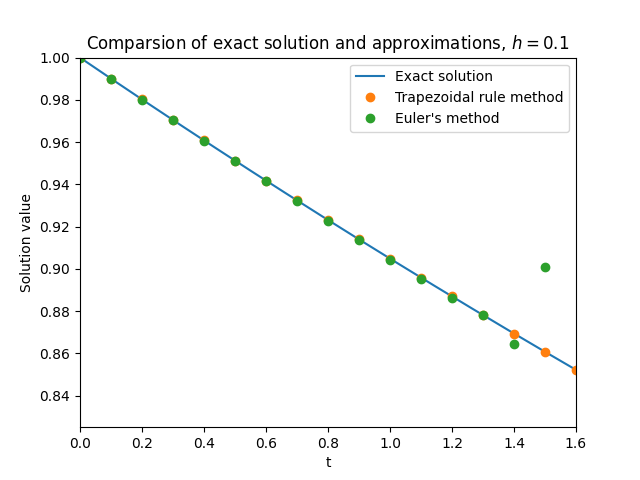
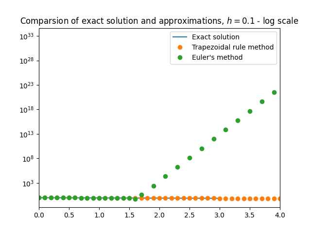
\(\text{ }\)Rounding error. If \(y_{0}\) is picked so that \(x_{1}=0,\) then in theory Euler’s method produces approximations \(y_{n}=x_{2}\left(1-\frac{h}{10}\right)^{n}\) and is “stable” even for the larger step-sizes up to \(h<20.\) But in practice rounding errors arise when computing \(y_{n}\) on a real computer using floating point arithmetic, and these can easily cause the approximation \(y_{n}\) to pick up a non-zero component in the \(x_{1}\) direction at some step \(m\) of the calculation, so that \(y_{m}=\varepsilon x_{1}+x_{2}\left(1-\frac{h}{10}\right)^{m}\) for some \(\varepsilon>0.\) The subsequent approximations will then equal \[y_{n}=\varepsilon x_{1}(1-100h)^{n-m}+x_{2}\left(1-\frac{h}{10}\right)^{n},\] and if \(h>\frac{1}{50}\) the first term will soon dominate the numerical solution. Figure Figure 12.1 shows this phenomenon in action.

Thus the only way to accurately approximate the solution with Euler’s method is to use a step-size \(h<\frac{1}{50},\) to accommodate the larger “nuisance” eigenvalue. ODEs that exhibit this kind of behavior are called stiff.

The source of the problem is not the local error: the method is of order \(1\) and the local error decays as \(O(h^{2})\) (i.e. Lemma 9.6

Lemma 9.6 ➔

Euler’s method from Definition 9.1 is of order \(p=1.\)

and ([eq:ch9_euler_order_lemma_proof_estimate]) still apply). Rather it is the inherent instability of the solutions ([eq:ch12_stiff_exact_euler_sol_x1_x2]) of the difference equation ([eq:ch12_stiff_ode_euler_diff_eq]) that causes stiffness. Note that this behavior does not contradict the fact that Euler’s method is convergent, as proved in Theorem 9.8

Theorem 9.8 ➔

Euler’s method from Definition 9.1 is convergent.

, since the latter only claims that the error converges to zero as \(h\downarrow0,\) without making any claim about the error for any particular \(h.\) The analysis here shows that one needs \(h<\frac{1}{50}\) for a reasonable approximation, which is however much smaller than the step-size that would suffice without the larger “nuisance” eigenvalue.

\(\text{ }\)Success of trapezoidal rule method. Let us now investigate the performance of the trapezoidal rule method applied to the IVP ([eq:ch12_stiff_ode_first_example]). Specializing the rule ([eq:ch9_trap_intro_rule]) to this ODE yields the implicit equation \[y_{n+1}=y_{n}+\frac{h}{2}(Ay_{n}+Ay_{n+1})\tag{12.8}\] for \(y_{n+1}\) in terms of \(y_{n}.\) In this simple case the equation can in fact be explicitly solved provided \(I-\frac{h}{2}A\) is non-degenerate, yielding \[y_{n+1}=\left(I-\frac{h}{2}A\right)^{-1}\left(I+\frac{h}{2}A\right)y_{n}.\] The approximations produced by the method are thus \[y_{n}=B^{n}y_{0}\quad\quad\text{where}\quad\quad B=\left(I-\frac{h}{2}A\right)^{-1}\left(I+\frac{h}{2}A\right).\] The basis that diagonalizes \(A\) also diagonalizes \(B,\) and \[\left(I-\frac{h}{2}D\right)^{-1}\left(I+\frac{h}{2}D\right)=\left(\begin{matrix}\frac{1-\frac{h}{2}100}{1+\frac{h}{2}100} & 0\\ 0 & \frac{1-\frac{h}{2}\frac{1}{10}}{1+\frac{h}{2}\frac{1}{10}} \end{matrix}\right),\] so \[B=V\left(\begin{matrix}\frac{1-\frac{h}{2}100}{1+\frac{h}{2}100} & 0\\ 0 & \frac{1-\frac{h}{2}\frac{1}{10}}{1+\frac{h}{2}\frac{1}{10}} \end{matrix}\right)V^{-1}.\] Therefore the approximations of the trapezoidal rule method can be written as \[y_{n}=V\left(\begin{matrix}\left(\frac{1-\frac{h}{2}100}{1+\frac{h}{2}100}\right)^{n} & 0\\ 0 & \left(\frac{1-\frac{h}{2}\frac{1}{10}}{1+\frac{h}{2}\frac{1}{10}}\right)^{n} \end{matrix}\right)V^{-1}y_{0}=x_{1}\left(\frac{1-\frac{h}{2}100}{1+\frac{h}{2}100}\right)^{n}+x_{2}\left(\frac{1-\frac{h}{2}\frac{1}{10}}{1+\frac{h}{2}\frac{1}{10}}\right)^{n}.\] Now the terms on the r.h.s. converge to \(0\) as \(n\to\infty,\) provided \[\left|\frac{1-\frac{h}{2}100}{1+\frac{h}{2}100}\right|<1\quad\quad\text{and}\quad\quad\left|\frac{1-\frac{h}{2}\frac{1}{10}}{1+\frac{h}{2}\frac{1}{10}}\right|<1.\tag{12.9}\] Since \[1\ge\frac{1-\frac{h}{2}100}{1+\frac{h}{2}100}=1-\frac{h100}{1+\frac{h}{2}100}>1-\frac{h100}{\frac{h}{2}100}=-1,\] we see that both inequalities in ([eq:ch12_stiff_trap_stability_cond]) in fact hold for all \(h>0\)! Thus the difference equation ([eq:ch12_stiff_ode_trap_diff_eq]) has “stable” solutions for any \(h>0,\) so one only needs to pick \(h>0\) small enough to ensure sufficiently small local error to obtain a good approximation. Instability is not an issue. Figure Figure 12.1 shows the approximations of ([eq:ch12_stiff_ode_first_example]) for \(h=0.1.\)

\(\text{ }\)Situations that lead to stiffness. It is hard to make a mathematically precise definition of stiffness. In general stiffness tends to happen when a system evolves at several time-scales of very different magnitude. The two terms ([eq:ch12_stiff_exact_sol_x1_x2]) in the ODE are an example of this, the “nuisance” term decays at a rate that is \(1000\) times faster than that of the main term. Another way to put it is that \(A\) has a large condition number (=ratio of largest to smallest eigenvalue). In this context the condition number is sometimes called the stiffness ratio. For an non-linear ODE the stiffness ratio can be defined as the condition number of the Jacobian in \(y\) of its function \(F\) (for the ODE ([eq:ch12_stiff_ode_first_example]) the Jacobian is \(A\)). This is justified by the observation that if one linearizes a non-linear ODE in a small neighborhood of a certain point in time, one obtains exactly an equation like ([eq:ch12_stiff_ode_first_example]) with the Jacobian in place of \(A\) (possibly in addition to a constant term). It is by no means guaranteed that such linearization actually captures the true behavior of solutions of the non-linear ODE, so one can not rely blindly on properties of the Jacobian to diagnose stiffness.

12.2 Linear stability domain and \(A\)-stability

One way to characterize the the sensitivity to stiffness of a general numerical method is through its linear stability domain.

\(\text{ }\)Linear stability domain. Imagine applying a general numerical method to the \(\mathbb{C}\)-valued IVP \[y'=\lambda y,\quad t\ge0,\quad\quad y(0)=1,\tag{12.11}\] for a complex number \(\lambda.\) The exact solution is \(y(t)=e^{\lambda t},\) which tends to zero as \(t\to\infty\) for any \(\lambda\) with \(\mathrm{Re}\lambda<0.\) A numerical method with a given step-size applied to the IVP may or may not produces approximations \(y_{n}\) such that \(y_{n}\to0.\) The linear stability domain is defined as the subset \(\mathcal{D}\subset\mathbb{C}\) of the complex plane, so that if the coefficient \(\lambda\) and step-size \(h\) are such that \(h\lambda\in\mathcal{D},\) then the approximations satisfy \(y_{n}\to0.\)

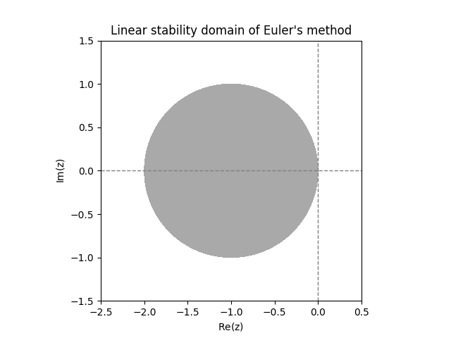
\(\text{ }\)Linear stability domain of Euler’s method. Applied to the IVP ([eq:linear_stabiility_domain_test_ODE]) Euler’s method produces the approximations \[y_{n}=(1+h\lambda)^{n}.\] Note that for a complex number \(a=re^{i\theta}\) we have \(a^{n}=r^{n}e^{in\theta},\) which tends to zero only if \(r<1.\) Thus \(y_{n}\) converges to zero only if \(\left|1+h\lambda\right|<1.\) Thus the linear stability domain of Euler’s method is \[\mathcal{D}=\left\{ z\in\mathbb{C}:\left|1+z\right|<1\right\} .\] This is the open ball of unit radius centered at \(-1\) (see Figure Figure 12.2).

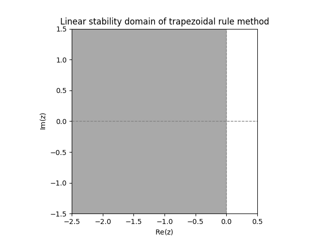
\(\text{ }\)Linear stability domain of the trapezoidal rule method. Applying the trapezoidal rule method to the IVP ([eq:linear_stabiility_domain_test_ODE]) yields \[y_{n}=\left(\frac{1+\frac{1}{2}h\lambda}{1-\frac{1}{2}h\lambda}\right)^{n}.\tag{12.12}\] This tends to zero iff \(\left|\frac{1+\frac{1}{2}h\lambda}{1-\frac{1}{2}h\lambda}\right|<1,\) so the linear stability domain is \[\mathcal{D}=\left\{ z\in\mathbb{C}:\frac{\left|1+\frac{z}{2}\right|}{\left|1-\frac{z}{2}\right|}<1\right\} .\tag{12.13}\] Since \[\frac{\left|1+\frac{z}{2}\right|}{\left|1-\frac{z}{2}\right|}=\frac{\left(1+\frac{\mathrm{Re}z}{2}\right)^{2}+\left(\frac{\mathrm{Im}z}{2}\right)^{2}}{\left(1-\frac{\mathrm{Re}z}{2}\right)^{2}+\left(\frac{\mathrm{Im}z}{2}\right)^{2}}\] and the r.h.s. is \(<1\) precisely when \(\mathrm{Re}z<0,\) we see that \[\mathcal{D}=\left\{ z\in\mathbb{C}:\mathrm{Re}z<0\right\} \tag{12.14}\] (see Figure Figure 12.2). The trapezoidal rule has a much larger linear stability domain than Euler’s method.

\(\text{ }\)Relevance of the linear stability domain for stiffness Imagine a \(\mathbb{R}^{d}\)-valued linear autonomous ODE \[\dot{y}=Ay,\quad t\ge0,\quad y(0)=y_{0},\tag{12.15}\] for a diagonalizable \(A\) with eigenvalues \(\lambda_{1},\ldots,\lambda_{n}\in\mathbb{C}\) with negative real part and \(y_{0}\in\mathbb{R}^{d}.\) When Euler’s method is applied to this ODE it produces \[y_{n}=(I+hA)^{n}y_{0}.\] In the basis where \(A\) is diagonal the matrix in that expression takes the form \((I+h{\rm Diag}(\lambda_{1},\ldots,\lambda_{d}))^{n},\) which means that the solutions produced are of the form \[y_{n}=x_{1}(1+h\lambda_{1})^{n}+\ldots+x_{d}(1+h\lambda_{d})^{n}\tag{12.16}\] for some \(x_{1},\ldots,x_{d}.\) Each term on the r.h.s. is the approximation by Euler’s method of the scalar ODE \[\dot{y}=\lambda_{i}y,\quad t\ge0,\quad y(0)=x_{i},\tag{12.17}\] for some \(i=1,\ldots,d.\) Similarly the trapezoidal rule method applied to ([eq:linear_stabiility_domain_d_dim_IVP]) yields \[y_{n}=x_{1}\left(\frac{1+\frac{h}{2}\lambda_{1}}{1-\frac{h}{2}\lambda_{1}}\right)^{n}+\ldots+x_{d}\left(\frac{1+\frac{h}{2}\lambda_{d}}{1-\frac{h}{2}\lambda_{d}}\right)^{n}\tag{12.18}\] for some \(x_{1},\ldots,x_{d},\) where each term on the r.h.s. is the approximation of the trapezoidal rule method applied to the scalar ODE ([eq:linear_stabiility_domain_d_dim_IVP_to_scalar]).

Note that ([eq:linear_stabiility_domain_d_dim_IVP_eul_sol]) resp. ([eq:linear_stabiility_domain_d_dim_IVP_trap_sol]) will be numerically unstable if at least one of the terms in ([eq:linear_stabiility_domain_d_dim_IVP_eul_sol]) resp. ([eq:linear_stabiility_domain_d_dim_IVP_trap_sol]) diverge, i.e. if \(h\lambda_{i}\notin\mathcal{D}\) for at least one \(i.\) That is, the “stiffest” component of the system determines stability or lack thereof. Therefore one might as well only consider the stiffest component, which is a scalar ODE like ([eq:linear_stabiility_domain_test_ODE]).

\(\text{ }\)A-stability. Any method whose linear stability in domain includes the half-plane \(\left\{ z\in\mathbb{C}:\mathrm{Re}z<0\right\}\) is called \(A\)-stable. Thus Euler’s method is not \(A\)-stable, while the trapezoidal rule method is.

12.3 Linear stability domain of Runge-Kutta methods

When applying the general \(k\)-stage Runge-Kutta method ([eq:ch11_IRK_general_form]) to ([eq:linear_stabiility_domain_test_ODE]) the intermediate stages \(\xi_{1},\ldots,\xi_{k}\) are determined by the equations \[\xi_{l}=y_{n}+h\sum_{i=1}^{k}a_{l,i}\lambda\xi_{i},\quad\quad l=1,\ldots,k.\] Letting \(A\) denote the Runge-Kutta matrix and \(\xi=(\xi_{1},\ldots,\xi_{k})\in\mathbb{R}^{k}\) and \({\bf 1}=(1,\ldots,1)\in\mathbb{R}^{k},\) we can write this in vector notation as \[\xi=y_{n}{\bf 1}+h\lambda A\xi.\] In this simple case this is a linear equation in \(\xi,\) which is easily solved explicitly as \[\xi=(I-h\lambda A)^{-1}{\bf 1}y_{n},\] (provide \(I-h\lambda A\) is invertible). The approximation produced for \(t=t_{n+1}\) is then \[\begin{array}{ccccl} y_{n+1} & = & y_{n}+h\sum_{i=1}^{k}b_{i}\lambda\xi_{i} & = & y_{n}+h\lambda b^{T}\xi\\ & & & = & y_{n}+h\lambda b^{T}(I-h\lambda A)^{-1}{\bf 1}y_{n}.\\ & & & = & \left(I+h\lambda b^{T}(I-h\lambda A)^{-1}{\bf 1}\right)y_{n}. \end{array}\] From this we obtain the explicit formula \[y_{n}=\left(I+h\lambda b^{T}(I-h\lambda A)^{-1}{\bf 1}\right)^{n}\tag{12.19}\] for the approximation at any \(t_{n}.\) This tends to zero as long as \[\left|I+h\lambda b^{T}\left(I-h\lambda A\right)^{-1}{\bf 1}\right|<1.\] The linear stability domain is therefore \[\mathcal{D}=\left\{ z\in\mathbb{C}:\left|r(z)\right|<1\right\} \quad\quad\text{for}\quad\quad r(z)=1+zb^{T}\left(I-zA\right)^{-1}{\bf 1}.\tag{12.20}\] Note that the numerical solution ([eq:ch12_stiff_RK_on_scalar_linear_sol_long]) can also be written in terms of \(r,\) namely \[y_{n}=r(h\lambda)^{n}.\tag{12.21}\]

\(\text{ }\)Examples of linear stability domains of ERKs. Using a computer it is easy to plot the stability region for any \(A\) and \(b.\) Figure Figure 12.3 shows the numerically computed linear stability domains of the three \(2\)-stage ERKs from ([eq:ch11_ERK_common_two_stage_methods]).

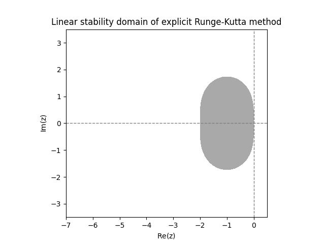
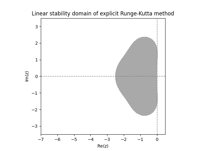
The three plots in Figure Figure 12.3 look suspiciously similar. In fact, it turns out that the functions \(r(z)\) for all three methods coincide, so they have exactly the same linear stability domain. Below we will explain why this happens. The next two plots show the linear stability domain of the \(3\)-stage ERKs from ([eq:ch11_ERK_common_three_stage]). Again they are actually identical.

\(\text{ }\)Examples of linear stability domains of IRKs. Turning to implicit Runge-Kutta methods, the next plot shows the linear stability domains of the \(2\)-stage IRK method ([eq:ch11_2_stage_IRK_example]) and the Gauss-Legendre \(2\)-stage IRK ([eq:ch11_2_state_gauss_lengendre_IRK]).

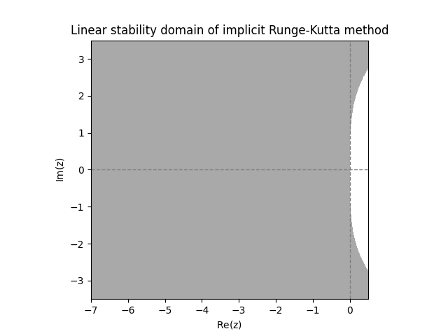
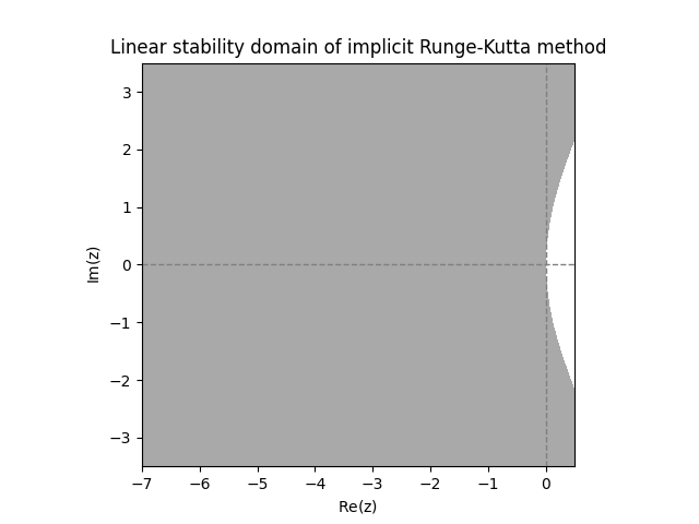
Examining the above diagrams, we see that the ERKs have quite a small linear stability domain, and have no chance of being \(A\)-stable. Both IRKs however appear to be \(A\)-stable.

One may note that some of these methods have a linear stability domain that covers part of the complex plane with non-negative real part. This is not actually an advantage, because there the true solution of ([eq:linear_stabiility_domain_test_ODE]) diverges, while the numerical solution converges to zero.

\(\text{ }\)Studying stability domains analytically. We now introduce some machinery that will allow us to investigate linear stability domains analytically. The first lemma proves that the quantity \(r(z)\) from ([eq:ch12_stiff_RK_D_and_r_def]) is a rational polynomial in \(z,\) and for ERKs just a polynomial. Recall that a rational polynomial is the ratio \(p(z)/q(z)\) for two polynomials \(p(z),q(z).\)

With this we can prove that ERKs are never \(A\)-stable.

\(\text{ }\)Polynomial \(r(z)\) of specific IRK. Turning to the IRK from ([eq:ch11_2_stage_IRK_example]), let us compute its polynomial \(r(z).\) By ([eq:linear_stabiility_domain_r_as_adj]) it equals \[\frac{\det(I-zA)+zb^{T}{\rm adj}(I-zA){\bf 1}}{\det(I-zA)}.\] We have \[\det(I-zA)=\left(1-\frac{z}{4}\right)\left(1-\frac{5}{12}z\right)-\left(-\frac{z}{4}\right)\left(\frac{z}{4}\right)=1-\frac{2}{3}z+\frac{z^{2}}{6},\] and \[{\rm adj}(I-zA)=\left(\begin{matrix}1-\frac{5}{12}z & -\frac{z}{4}\\ \frac{z}{4} & 1-\frac{z}{4} \end{matrix}\right),\] so \[b^{T}{\rm adj}(I-zA){\bf 1}=\frac{1}{4}\left(1-\frac{5}{12}z-\frac{z}{4}\right)+\frac{3}{4}\left(\frac{z}{4}+1-\frac{z}{4}\right)=1-\frac{z}{6},\] and \[r(z)=\frac{1-\frac{2}{3}z+\frac{z^{2}}{6}+z-\frac{1}{6}z^{2}}{1-\frac{2}{3}z+\frac{1}{6}z^{2}}=\frac{1+\frac{1}{3}z}{1-\frac{2}{3}z+\frac{1}{6}z^{2}}.\tag{12.24}\] It is possible to use “brute-force calculation” to prove that for this \(r\) it holds that \(|r(z)|<1\) for all \(z\) with negative imaginary part. However, it is easier to instead verify the criterion of the next lemma, which is equivalent to the latter statement.

Applying this to ([eq:linear_stabiility_domain_IRK_poly_r]), we first note that any poles are roots of the quadratic \(1-\frac{2}{3}z+\frac{1}{6}z^{2}.\) It factors as \((z-(2-i\sqrt{2}))(z-(2+i\sqrt{2})),\) so both roots have positive imaginary part, so all poles of \(r(z)\) have positive real part. It only remains to consider \(r(z)\) for purely imaginary \(z,\) i.e. \(z=it\) for \(t\in\mathbb{R}.\) We have \[\begin{array}{ccccccc} |r(it)| & = & \frac{\left|1+\frac{1}{3}it\right|}{\left|1-\frac{2}{3}it-\frac{1}{6}t^{2}\right|} & = & \frac{\sqrt{1+\frac{1}{9}t^{2}}}{\sqrt{\left(1-\frac{1}{6}t^{2}\right)^{2}+\frac{4}{9}t^{2}}} & = & \frac{\sqrt{1+\frac{1}{9}t^{2}}}{\sqrt{1-\frac{1}{3}t^{2}+\frac{1}{36}t^{4}+\frac{4}{9}t^{2}}}\\ & & & & & = & \frac{\sqrt{1+\frac{1}{9}t^{2}}}{\sqrt{1+\frac{1}{9}t^{2}+\frac{1}{36}t^{4}}}<1. \end{array}\] This proves that the IRK method from ([eq:ch11_2_stage_IRK_example]) is \(A\)-stable.

The following lemma further restricts the possible forms \(r(z)\) can take.

This explains why the linear stability domains of ERKs with the same number stages in Figure Figure 12.3 and Figure Figure 12.4 are identical: they are explicit methods, so by Lemma 12.1

Lemma 12.1 ➔

Let \(k\ge1.\) For any matrix \(A\in\mathbb{R}^{k\times k}\) and vector \(b\in\mathbb{R}^{k}\) the function \[r(z)=1+zb^{T}\left(I-zA\right)^{-1}{\bf 1}\tag{12.22}\] is the ratio of two polynomials of degree at most \(k.\) If \(A\) is strictly lower triangular, then \(r(z)\) is a polynomial of degree at most \(k.\)

the function \(r(z)\) is simply a polynomial of order at most \(k.\) Thus the \(r(z)\) of the \(k=2\)-stage methods are quadratic. The methods are also of order \(p=2,\) so the previous lemma implies that \(r(z)=e^{z}+O(z^{3}).\) Only one quadratic satisfies this, namely the polynomial \(r(z)=1+z+\frac{z^{2}}{2},\) which comes from truncating the Taylor series of \(e^{z}.\) This proves that the linear stability domains in Figure Figure 12.3 must necessarily agree. Similarly, for \(k=3\)-stages \(r(z)\) is a cubic, and the ERKs in Figure Figure 12.3 are of order \(p=3,\) so \(r(z)=e^{z}+O(z^{4}),\) which can only happen for a cubic \(r(z)\) if \(r(z)=1+z+\frac{z^{2}}{2}+\frac{z^{3}}{6}.\) Again, this proves that the linear stability domains in Figure Figure 12.4 must agree.

We finish by stating without proof the following proposition guaranteeing that the Gauss-Legendre method with any number of stages is is \(A\)-stable.

In conclusion, we see that explicit RK method don’t have a very big linear stability domain, while implicit RK can achieve the gold standard - \(A\)-stability. Thus the higher computational complexity of implicit methods can be worth it, especially for stiff ODEs.

12.4 Linear stability domain of multistep methods

For an \(s\)-step multistep method we define the linear stability domain \(\mathcal{D}\) as the set of \(h\lambda\) such that the approximations \(y_{n}\) the method produces when approximating ([eq:linear_stabiility_domain_test_ODE]) tends to zero as \(n\to\infty,\) for all possible values of \(y_{1},\ldots,y_{s-1}.\)

\(\text{ }\)Deriving linear stability domain.The general \(s\)-step linear multistep method ([eq:ch9_general_multistep]) applied to the IVP ([eq:linear_stabiility_domain_test_ODE]) yields \[\sum_{m=0}^{s}a_{m}y_{n+m}=h\lambda\sum_{m=0}^{s}b_{m}y_{n+m}.\] Let us rewrite it as \[\sum_{m=0}^{s}(a_{m}-h\lambda b_{m})y_{n+m}=0.\] This is a linear difference equation, as studied in Section 10.3. Recall that the general solution of such a difference equation involves the roots of its characteristic polynomial \[p(w)=\sum_{m=0}^{s}(a_{m}-h\lambda b_{m})w^{m}.\] Indeed letting \(w_{1},\ldots,w_{k}\) be the distinct roots with respective multiplicities \(m_{1},\ldots,,m_{k},\) the formula for the general solution is \[y_{n}=\sum_{i=1}^{k}q_{i}(n)w_{i}^{n},\] where \(q_{i}\) is an arbitrary polynomial of degree at most \(m_{i}-1.\) The r.h.s. converges to zero as \(n\to\infty\) only if \(|w_{i}|<1\) for all \(i\) such that \(q_{i}\ne0.\) Since we allow for any possible starting values for \(y_{1},\ldots,y_{s-1}\) we can not assume that any of the \(q_{i}\) vanish. Thus the linear stability domain is \[\mathcal{D}=\left\{ z\in\mathbb{C}:\text{all roots of }\sum_{m=0}^{s}\left(a_{m}-zb_{m}\right)w^{m}\text{ have norm less than }1\right\}\] \(\text{ }\)Investigating linear stability domains graphically. Computing the roots numerically for a grid of \(z\)-s one can plot the linear stability domains of any fixed multistep method. The next figure shows the result for the Adams-Bashforth methods with \(s=2\) and \(s=3\) steps.

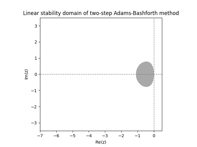
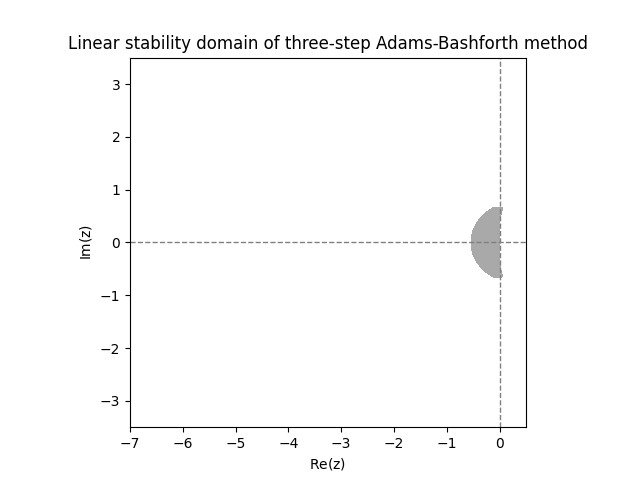
These linear stability domains are disappointingly small. The next figure shows the linear stability domains of Adams-Moulton methods with \(s=2\) and \(s=3\) steps.

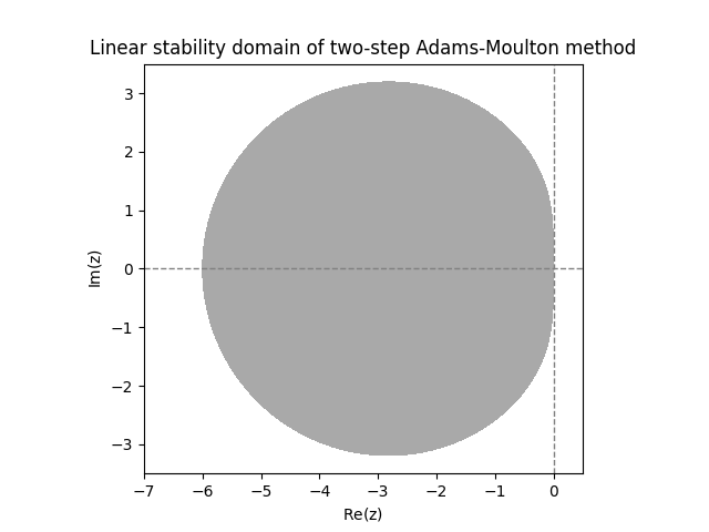
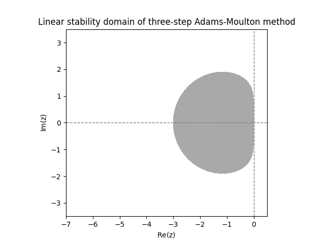
The implicit Adams-Moulton methods have a significantly larger linear stability domain, but are far from being \(A\)-stable. The next diagram shows linear stability domains for BDFs with \(s=2,3,4\) steps.

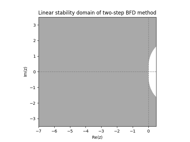
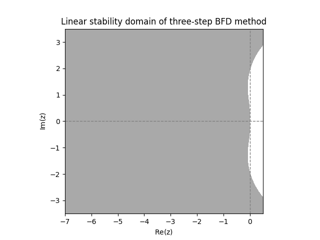
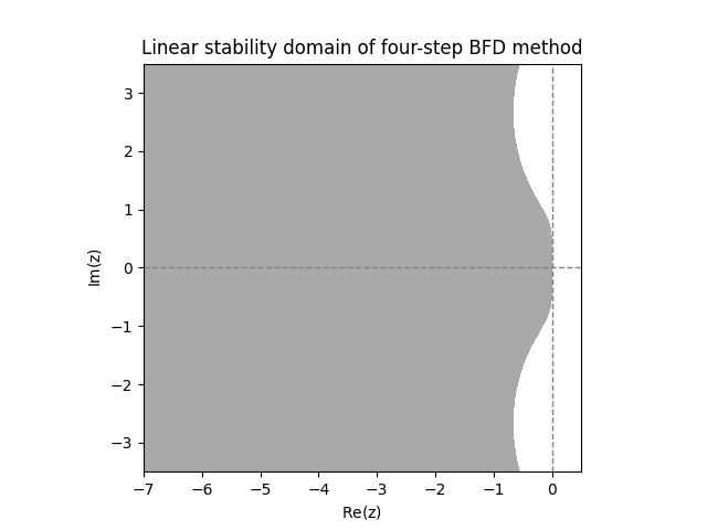
We observe much larger linear stability domains. For \(s=2\) steps it even looks like the method is \(A\)-stable. For \(s=3,4\) steps it appears that the methods are close to being \(A\)-stable, but not quite.

\(\text{ }\)Analytical results.

We record here without proof the theorem stating that the \(s=2\)-step BDF method is indeed \(A\)-stable.

Unfortunately no other convergent BDF is \(A\)-stable. Indeed the following “barrier theorem” for \(A\)-stability of multistep methods holds, which we state without proof.

While not \(A\)-stable, we see from Figure Figure 12.8 that the higher order BDFs do have quite a large linear stability domain. In particular they include a “wedge” of the form \[\left\{ -\rho e^{i\theta}:\rho>0\quad\quad\left|\theta\right|<\alpha\right\}\] for some \(\alpha>0.\) A method whose linear stability domain contains such a wedge is called \(A(\alpha)\)-stable. It turns out that the BDF methods with \(s=3,4,5,6\) steps are all \(A(\alpha)\)-stable.

Theory and Numerics of ODEs

Home

Contents

Weeks

---

✕