9.3 Trapezoidal rule method
The trapezoidal rule is a numerical method for approximating solutions to ODEs whose error decays faster in \(h\) than that of Euler’s method. Its heuristic derivation is based on the trapezoidal rule for approximating definite integrals like \(\int_{t_{0}}^{t_{\max}}f(t)dt\) by sums.
This is Sparta [sec:ch9_trap_rule_method].
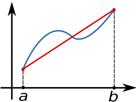
\(\text{ }\) Trapezoidal rule for Riemann sums. Recall from ([eq:ch9_def_int_riemann_err]) that the error bound in approximating an integral by the left Riemann sum \(h\sum_{n}f(t_{n})\) is linear in \(h.\) More precisely, \[\left|\int_{t_{0}}^{t_{\max}}f(t)dt-h\sum_{n=0}^{N-1}f(t_{n})\right|\le ch,\tag{9.24}\] for \(c=(t_{\max}-t_{0})\sup_{t\in[t_{0},t_{\max}]}\left|f''(t)\right|\) and \(t_{\max}=t_{0}+Nh.\) The left Riemann sum approximation arises from the approximation \(\int_{t_{n}}^{t_{n+1}}f(t)dt\approx hf(t_{n})\) for a small interval \([t_{n},t_{n+1}].\) The trapezoidal rule replaces this by the approximation \(\int_{t_{n}}^{t_{n+1}}f(t)dt\approx\int_{t_{n}}^{t_{n+1}}g(t)dt,\) where \(g(t)\) the linear interpolation such that \(g(t_{n})=f(t_{n}),g(t_{n+1})=f(t_{n+1})\) - see Figure Figure 9.2. It is easy to prove that \(\int_{t_{n}}^{t_{n+1}}g(t)dt=\frac{h}{2}\left(f(t_{n})+f(t_{n+1})\right)\) (exercise: prove it). Thus the trapezoidal rule approximates the integral over \([t_{n},t_{n+1}]\) as \[\int_{t_{n}}^{t_{n+1}}f(t)dt\approx h\frac{f(t_{n})+f(t_{n+1})}{2}.\tag{9.25}\] The approximation for the integral over the whole interval is then \[\int_{t_{0}}^{t_{\max}}f(t)dt\approx h\sum_{n=0}^{N-1}\frac{f(t_{n})+f(t_{n+1})}{2}.\tag{9.26}\]
The error in this approximation decays faster than linearly in \(h,\) i.e. faster than the r.h.s. of ([eq:ch9_trap_recall_left_riemann_err]) (provided \(f\) is twice continuously differentiable), as we now argue. Let us first consider the error for a single interval: \[\left|\int_{t_{n}}^{t_{n+1}}f(t)dt-h\frac{f(t_{n})+f(t_{n+1})}{2}\right|.\] To this end let \(G(t)=\int_{t_{n}}^{t}f(s)ds,\) so that the first term above is \(G(t_{n+1}),\) and note that by Taylor’s theorem \[G(t_{n+1})=G(t_{n})+hG'(t_{n})+\frac{h^{2}}{2}G''(t_{n})+O\left(h^{3}\sup_{t\in[t_{0},t_{\max}]}\left|G'''(t)\right|\right),\tag{9.27}\] if \(G\) is three times continuously differentiable, where we have used big \(O\) notation to compactly express that there is a universal constant \(c>0\) such that \[\left|G(t_{n+1})-\left\{ G(t_{n})+hG'(t_{n})+\frac{h^{2}}{2}G''(t_{n})\right\} \right|\le ch^{3}\sup_{t\in[t_{0},t_{\max}]}\left|G'''(t)\right|\] for any such \(G.\) By the definition of \(G\) this implies \[G(t_{n+1})=hf(t_{n})+\frac{h^{2}}{2}f'(t_{n})+O\left(h^{3}\sup_{t\in[t_{0},t_{\max}]}\left|f''(t)\right|\right)\tag{9.28}\] for all \(h>0\) and twice continuously differentiable functions \(f.\) Similarly under the same assumption \[f(t_{n+1})=f(t_{n})+hf'(t_{n})+O\left(h^{2}\sup_{t\in[t_{0},t_{\max}]}\left|f''(t)\right|\right).\] Thus \[h\frac{f(t_{n})+f(t_{n+1})}{2}=hf(t_{n})+\frac{h^{2}}{2}f'(t_{n})+O\left(h^{3}\sup_{t\in[t_{0},t_{\max}]}\left|f''(t)\right|\right).\tag{9.29}\] Comparing the r.h.s.s of ([eq:ch9_trapezoidal_integral_G-1]) and ([eq:ch9_trapezoidal_integral_heuristic_avg]) we see that the first two terms match, so that \[\int_{t_{n}}^{t_{n+1}}f(t)dt-h\frac{f(t_{n})+f(t_{n+1})}{2}=O\left(h^{3}\sup_{t\in[t_{0},t_{\max}]}\left|f''(t)\right|\right).\] The error bound for one interval is thus cubic in \(h\) for the trapezoidal rule, as opposed to quadratic for the left Riemann-sum (recall ([eq:ch9_def_int_riemann_err_one_step])). To bound the error for whole interval \([t_{0},t_{\max}]\) one simply sums this estimate over \(n=0,\ldots,N-1\) and uses that \(Nh^{3}=\frac{t_{\max}-t_{0}}{h}h^{3}=\left(t_{\max}-t_{0}\right)h^{2}\) to obtain \[\int_{t_{0}}^{t_{\max}}f(t)dt-h\sum_{n=0}^{N-1}\frac{f(t_{n})+f(t_{n+1})}{2}=O\left(h^{2}(t_{\max}-t_{0})\sup_{t\in[t_{0},t_{\max}]}\left|f''(t)\right|\right)\tag{9.30}\] The r.h.s. is quadratic in \(h,\) as opposed to linear like in ([eq:ch9_def_int_riemann_err]). That is, the trapezoidal rule for approximating definite integrals has a global error bound which decays quadratically in \(h,\) faster than the linear in \(h\) bound for the left Riemann sum. Assuming for simplicity that the prefactor of the power of \(h\) is equal to one in both cases, this means that to achieve an error bounded by \(\frac{1}{100}\) the left Riemann sum needs \(h=\frac{1}{100},\) while the trapezoidal rule sum needs only \(h=\frac{1}{10}\): or in other words, the left Riemann sum needs \(100\) summands to satisfy such a bound, while the trapezoidal rule sum needs only \(10.\)
\(\text{ }\) Trapezoidal rule method for ODEs. Inspired by this, we can build a numerical method for first order ODEs by applying the approximation ([eq:ch9_trap_heuristic_derivation_approx_one_interval]) to \(y_{n+1}-y_{n}=\int_{t_{n}}^{t_{n+1}}F(t,y(t))dt,\) yielding \[\int_{t_{n}}^{t_{n+1}}F(t,y(t))dt\approx h\frac{F(t_{n},y(t_{n}))+F(t_{n+1},y(t_{n+1}))}{2},\] and thus \[y_{n+1}=y_{n}+h\frac{F(t_{n},y_{n})+F(t_{n+1},y_{n+1})}{2}.\tag{9.31}\] The last equation is the trapezoidal rule method for numerically approximating solutions to ODEs. Note that it differs from Euler’s method ([eq:ch9_euler_method_def_one_step]) in that it specifies \(y_{n+1}\) in terms of \(y_{n}\) implicitly. That is, \(y_{n+1}\) is defined as a solution of the equation \[y=y_{n}+h\frac{F(t_{n},y_{n})+F(t_{n+1},y)}{2}.\tag{9.32}\] The next plot compares the exact solution of an ODE to the approximation by the trapezoid rule method and Euler’s method for the same step-size.
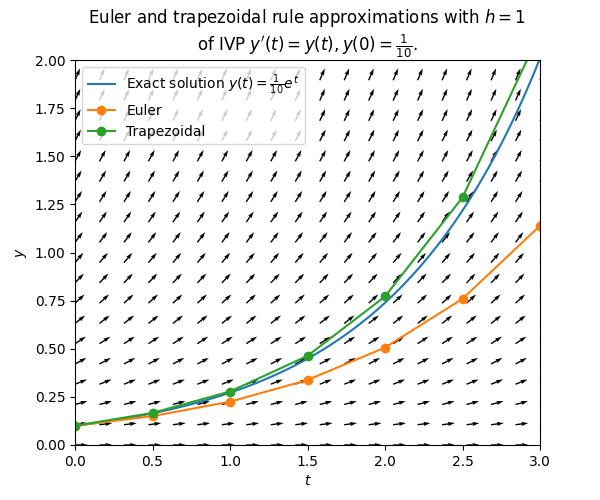
We see that in this case the error of the trapezoidal rule method is much smaller. Below we will prove error bounds for the trapezoidal rule method that decay faster in \(h\) than those for Euler’s method. One should keep in mind however, that the comparison is not entirely fair: for the same step-size \(h\) the trapezoidal rule method uses more computational resources, since it needs to solve the implicit equation ([eq:ch9_trapezoidal_heu_implicit_eq]) at each step.
The Jacobian is the matrix with entries \(\left(D_{y}G(h_{0},y_{0})\right)_{ij}=\partial_{y_{j}}G_{i}(h_{0},y_{0})\) for \(i,j=1,\ldots,d.\)
Assuming \(F\) is continuously differentiable and given \(t_{n},y_{n}\) we can define \[G(h,y)=y-y_{n}-h\frac{F(t_{n},y_{n})+F(t_{n+1},y)}{2}.\] This function satisfies \(G(0,y_{n})=0,\) and \(D_{y}G(h,y)=I-\frac{h}{2}D_{y}F(t_{n+1},y)\) implying \(D_{y}G(0,y_{n})=I,\) which is clearly non-degenerate. Therefore for each \(n\) there exists by the implicit function theorem some small enough \(c>0\) such that for any \(h\in(0,c)\) there exists a unique solution \(y\in\mathbb{R}^{d}\) of \(G(h,y)=0\) closest to \(y_{n},\) i.e. a closest solution of ([eq:ch9_trapezoidal_heu_implicit_eq]). Reassuringly, this means that for small enough \(h>0\) the implicit equation ([eq:ch9_trapezoidal_heu_implicit_eq]) defines a unique \(y_{n+1}.\)
Unfortunately, the standard version of the implicit function theorem does not provide a lower bound for the constant \(c>0\): this means that it cannot guarantee that for any single \(h>0\) the unique closest solution exists simultaneously for all steps \(n=0,1,2,\ldots\) of the method. The next section will deal with existence guarantees for all steps simultaneously.
\(\text{ }\) Formal definition. Let us now formally define the trapezoidal rule method.
Given \(d\ge1,\) \(V=\mathbb{R}^{d}\) or \(V=\mathbb{C}^{d},\) \(t_{0},t_{\max}\in\mathbb{R},t_{0}<t_{\max}\) , a function \(F:[t_{0},t_{\max}]\times V\to V,\) a \(y_{0}\in V\) and \(h>0,\) the trapezoidal rule method defines the approximations \(y_{n},1\le n\le\frac{t_{\max}-t_{0}}{h}\) as follows:
For \(n\ge0\) it defines \(y_{n+1}\) as the solution of \[y=y_{n}+h\frac{F(t_{n},y_{n})+F(t_{n+1},y)}{2}\tag{9.34}\] closest to \(y_{n},\) provided such a solution exists (breaking ties in some arbitrary way if there are several closest solutions). If no solution exists it defines \(y_{n+1}=y_{n}.\)
a) The part about breaking ties and the case when no solution exists are absolutely unimportant in practice, they are just there to make the definition formally complete.
A time-stepping method is a sequence of functions \[Y_{n}(F,h,t_{0},y_{0},y_{1},\ldots,y_{n})\quad\quad n=0,1,2,\ldots\] that take as input an \(F:[t_{0},t_{\max}]\times V\to V,\) where \(t_{0}\in\mathbb{R},t_{\max}\in\mathbb{R},t_{0}<t_{\max}\) and \(V=\mathbb{R}^{d}\) or \(V=\mathbb{C}^{d},\) and a step-size \(h>0,\) and outputs an element of \(V.\)
The output of the time-stepping method is the sequence \[y_{n+1}=Y_{n}(F,h,t_{0},y_{0},\ldots,y_{n})\quad\quad0\le n\le\frac{t_{\max}-t_{0}}{h}.\] If the IVP \[\dot{y}(t)=F(t,y(t)),\quad\quad t\in I,\quad\quad y(t_{0})=y_{0},\tag{9.11}\] has a unique solution \(y,\) then the errors of the method is \[e_{n}=y_{n}-y(t_{n})\quad\quad0\le n\le\frac{t_{\max}-t_{0}}{h}.\tag{9.12}\] The global error over the whole interval \([t_{0},t_{\max}]\) is \[\max_{0\le n\le\frac{t_{\max}-t_{0}}{h}}\left|e_{n}\right|.\]
c) As defined here this method is strictly speaking impossible to implement on a computer, since it defines \(y_{n+1}\) as the exact solution of ([eq:ch9_trapezoidal_rule_implicit_eq]). In practice, the solution can not be computed exactly (except in simple cases), only approximated. In the next section we consider the combination of the trapezoidal rule with an approximation algorithm for solving ([eq:ch9_trapezoidal_rule_implicit_eq]).
Let \(p\ge0.\) Assume a time-stepping method like in Definition 9.2 is such that for every analytic \(F\) and \(y_{0}\in V,n\ge1\) there are positive constants \(c_{1},c_{2}\) such that if \(h\in(0,c_{1}]\) then \[\left|y(t_{n+1})-Y_{n}(F,h,t_{0},y(t_{0}),y(t_{1}),\ldots,y_{n}(t_{n}))\right|\le c_{2}h^{p+1},\tag{9.14}\] whenever ([eq:ch9_numerical_time_stepping_def_IVP]) has a unique solution \(y(t)\) defined on \([0,t_{n+1}].\) Then we call it a \(p\)-th order method.
Given \(d\ge1,\) \(V=\mathbb{R}^{d}\) or \(V=\mathbb{C}^{d},\) \(t_{0},t_{\max}\in\mathbb{R},t_{0}<t_{\max}\) , a function \(F:[t_{0},t_{\max}]\times V\to V,\) a \(y_{0}\in V\) and \(h>0,\) the trapezoidal rule method defines the approximations \(y_{n},1\le n\le\frac{t_{\max}-t_{0}}{h}\) as follows:
For \(n\ge0\) it defines \(y_{n+1}\) as the solution of \[y=y_{n}+h\frac{F(t_{n},y_{n})+F(t_{n+1},y)}{2}\tag{9.34}\] closest to \(y_{n},\) provided such a solution exists (breaking ties in some arbitrary way if there are several closest solutions). If no solution exists it defines \(y_{n+1}=y_{n}.\)
Proof. Recall that \(V=\mathbb{R}^{d}\) or \(V=\mathbb{C}^{d},\) and \(F\) is assumed to be analytic. For the present method the l.h.s. of ([eq:ch9_time_stepping_method_order_local_err]) equals \[\left|y(t_{n+1})-y_{n+1}\right|,\] where \(y_{n+1}\) is a solution to \[y=y(t_{n})+h\frac{F(t_{n},y(t_{n}))+F(t_{n+1},y)}{2}\tag{9.35}\] closest to \(y_{n}\) (if such a solution exists).
Let \[G:[0,1]\times V\to V\] be defined by \[G(h,y)=y-y_{n}-h\frac{F(t_{n},y(t_{n}))+F(t_{n+1},y_{n+1})}{2}.\] Since \(F\) is analytic \(G(h,y)\) is infinitely differentiable. Furthermore \(G(0,y_{n})=0,\) and \(D_{y}G(0,y_{n})=I,\) so the implicit function theorem implies that there exists \(0<\overline{c}_{1}\le1,\) \(\overline{c}_{2}>0\) and a continuous function \(y:[0,\overline{c}_{1}]\to V\) such that \[\begin{array}{c} h\in[0,\overline{c}_{1}],\left|y-y_{n}\right|\le\overline{c}_{2}\quad\quad\text{and}\quad\quad G(h,y)=0\\ \iff\\ h\in[0,\overline{c}_{1}],\left|y-y_{n}\right|\le\overline{c}_{2}\quad\quad\text{and}\quad\quad y=y(h). \end{array}\] This implies that for \(h\in(0,\overline{c}_{1}]\) there is indeed a unique solution \(y_{n+1}\) of ([eq:ch9_thm_trap_order_2_implicit_eq]) closest to \(y_{n}.\)
Let \(d\ge1,\) and \(V=\mathbb{R}^{d}\) or \(V=\mathbb{C}^{d}.\) Let \(t_{0},t_{\max}\in\mathbb{R},t_{0}<t_{\max}\) and \(I=[t_{0},t_{\max}].\) Let \(F:I\times V\to V\) and \(y_{0}\in V.\) Let \(h>0.\) Assume that \(F\) is analytic. If the IVP \[\dot{y}(t)=F(t,y(t)),\quad\quad t\in I,\quad\quad y(t_{0})=y_{0},\tag{9.16}\] has a solution \(y:I\to V,\) then \(y\) is analytic.
Euler’s method from Definition 9.1 is of order \(p=1.\)
\(\text{ }\) Generalization of Euler and Trapezoidal rule methods. Both Euler’s method and the trapezoidal rule method are of the form \[y_{n+1}=y_{n}+h\left(\theta F(t_{n},y_{n})+(1-\theta)F(t_{n+1},y_{n+1})\right)\tag{9.42}\] for \(\theta\in[0,1].\) Euler’s method corresponds to \(\theta=1\) and the trapezoidal rule method to \(\theta=\frac{1}{2}.\) A general method of this type is called a theta method. For \(\theta=1\) (i.e. Euler) the method is explicit, for all other \(\theta\) it is implicit.
Beyond the two we have already seen, the most important theta method corresponds to \(\theta=1,\) i.e. \[y_{n+1}=y_{n}+hF(t_{n+1},y_{n+1}),\] where \(y_{n}\) doesn’t appear at all in the second term of the r.h.s. This method can variously be referred to as the implicit Euler method or the backward Euler method. By constrast Euler’s method with \(\theta=1\) (i.e. ([eq:ch9_euler_method_def_one_step])) is sometimes called the explicit Euler method or the forward Euler method.
9.4 Fixed-point equations
In this section we
investigate guarantees for the existence of solutions to implicit equations that can be used to prove the global convergence of implicit methods, such as the trapezoidal rule method of the previous section,
investigate guarantees on the numerical solution of such implicit equations using simple fixed-point iteration,
prove the global convergence of the trapezoidal rule method.
\(\text{ }\)General class of fixed-point equations. To this end we investigate implicit equations of the form \[w=hg(w)+\beta\tag{9.44}\] where \(h>0,\) \(\beta\in V\) and \(g:V\to V\) for \(V=\mathbb{R}^{d}\) or \(V=\mathbb{C}^{d}.\) The implicit equation ([eq:ch9_trapezoidal_rule_implicit_eq]) of the trapezoidal rule method is of this form with \(\beta=y_{n}\) and \(g(w)=\frac{1}{2}\left(F(t_{n},y_{n})+F(t_{n+1},w)\right).\)
\(\text{ }\)Iterative solution The obvious iterative algorithm to solve this equation is to start with some \(w_{0},\) and compute \[w_{n+1}=hg(w_{n})+\beta,n\ge0.\] For “good” \(g,\beta,h\) one may hope that this sequence converges as \(n\to\infty.\) If so, the r.h.s. converges to its limit \(w,\) and if \(g\) is continuous the l.h.s. converges to \(hg(w)+\beta,\) so the limit \(w\) satisfies \(w=hg(w)+\beta\) and is thus a solution of ([eq:ch9_fixed_point_eq_general_eq]).
Since a computer can only make a finite number of computations, a practical implementation must have a rule for how to stop the iteration. The last value of \(w_{n}\) is then outputted as an approximation of the true solution. For instance on can stop after a fixed number of steps \(N,\) e.g. \(N=3,N=10,N=100,N=1000.\) Alternatively one can specify a tolerance level \(\varepsilon>0,\) e.g. \(\varepsilon=10^{-1},10^{-2},10^{-3},\ldots\) and stop once \[\left|w_{n}-hg(w_{n})-\beta\right|\le\varepsilon.\]
\(\text{ }\)Convergence guarantee. The next theorem gives conditions under which the sequence \(w_{n}\) converges. It is essentially a version of the famous Banach fixed-point theorem.
Let \(d\ge1\) and \(V=\mathbb{R}^{d}\) or \(V=\mathbb{C}^{d}.\) For \(w\in V\) and \(r\ge0\) define the closed ball \(B(w,r)=\left\{ v\in V:\left|v-w\right|\le r\right\} .\) Let \(g:V\to V.\) Let \(w_{0}\in V,\beta\in V,\rho>0,h>0\) and define the sequence \[w_{n+1}=hg(w_{n})+\beta,n\ge0.\tag{9.46}\] Assume that
\(g\) is continuous on \(B(w_{0},\rho),\) and
for all \(u,v\in B(w_{0},\rho)\) it holds that \(\left|g(u)-g(v)\right|\le\frac{\lambda}{h}\left|u-v\right|,\) and
\(\left|w_{1}-w_{0}\right|\le(1-\lambda)\rho.\)
Then
\(w_{n}\in B(w_{0},\rho)\) for all \(n\ge0,\) and
the sequence \(w_{n}\) is convergent, and \(w_{n}\to w_{\infty}\in B(w_{0},\rho),\) and
the limit \(w_{\infty}\) solves \[w=hg(w)+\beta,\tag{9.47}\] and is the unique solution to ([eq:ch9_banach_fixed_point_fixed_point_eq]) in \(B(w_{0},\rho\)).
Proof. We first prove (1). Assume for contradiction that this is not the case, and let \(n\) be s.t. \(w_{n+1}\) is the first iterate not in \(B(w_{0},\rho).\) That is, \[w_{m}\in B(w_{0},\rho)\text{ for all }m\le n\text{ and }w_{n+1}\notin B(w_{0},\rho).\tag{9.48}\] Using the definition ([eq:ch9_banach_fixed_point_thm_iteration]) and hypothesis (b) it holds that \[\left|w_{n+1}-w_{n}\right|=\left|hg(w_{n})-hg(w_{n-1})\right|=h\left|g(w_{n})-g(w_{n-1})\right|\le\lambda\left|w_{n}-w_{n-1}\right|.\tag{9.49}\] This inequality can be iterated since we have assumed that \(w_{m}\in B(w_{0},\rho)\) for all \(m\le n,\) so we obtain using also hypothesis (c) that \[\left|w_{m+1}-w_{m}\right|\le\lambda^{m}\left|w_{1}-w_{0}\right|\le\lambda^{m}(1-\lambda)\rho\quad\text{for all }\quad m\le n.\tag{9.50}\] Thus since \(0<\lambda<1\) \[\left|w_{n+1}-w_{0}\right|\le\sum_{m=0}^{n}\left|w_{m+1}-w_{m}\right|\le\sum_{m=0}^{n}\lambda^{m}(1-\lambda)\rho\le\sum_{m=0}^{\infty}\lambda^{n}(1-\lambda)\rho=\rho.\] But this contradicts ([eq:ch9_banach_fixed_point_thm_assume_for_contradiction]). Thus \(w_{n}\in B(w_{0},\rho)\) for all \(n\ge0,\) proving (1).
To prove (2), note that since \(w_{n}\in B(w_{0},\rho)\) for all \(n\ge0\) the inequality ([eq:ch9_banach_fixed_point_thm_increment_bound]) holds for all \(m,\) i.e. \[\left|w_{n+1}-w_{n}\right|\le\lambda^{n}(1-\lambda)\rho\quad\text{ for all }\quad n\ge0.\] Thus \[\sum_{n=0}^{\infty}\left|w_{n+1}-w_{n}\right|\le\sum_{m=0}^{\infty}\lambda^{n}(1-\lambda)\rho<\infty,\] so the sum \(\sum_{n=0}^{\infty}(w_{n+1}-w_{n})\) is absolutely convergent. Therefore there exists a \(w'\in V\) such that \[w'=\lim_{m\to\infty}\sum_{n=0}^{m}\left(w_{n+1}-w_{n}\right)=\sum_{n=0}^{\infty}(w_{n+1}-w_{n}).\] Let \(w_{\infty}=w'+w_{0}.\) Since \(\sum_{n=0}^{m}(w_{n+1}-w_{n})=w_{m+1}-w_{0}\) we have \[\lim_{n\to\infty}w_{n}=w_{\infty}.\] Since \(w_{n}\in B(w_{0},\rho)\) for all \(n\ge0\) and the ball \(B(w_{0},\rho)\) is closed, then also \(w_{\infty}\in B(w_{0},\rho).\) This proves (2).
Turning to (3), since \(g\) is continuous it holds that \[\lim_{n\to\infty}\left(hg(w_{n})+\beta\right)\to hg(w_{\infty})+\beta,\] which proves that \[w_{\infty}=hg(w_{\infty})+\beta.\tag{9.51}\] Lastly, assume that \(v\) is a different solution to ([eq:ch9_banach_fixed_point_fixed_point_eq_in_proof]) in \(B(w_{0},\rho).\) Then by hypothesis (b) \[\left|w_{\infty}-v\right|=h\left|g(w_{\infty})-g(v)\right|\le\lambda\left|w_{\infty}-v\right|<\left|w_{\infty}-v\right|,\] which is a contradiction, proving the uniqueness of the solution \(w_{\infty}.\)
A numerical time-stepping method such that \[\lim_{h\downarrow0}\max_{0\le n\le\frac{t_{\max}-t_{0}}{h}}|e_{n}^{h}|=0\] whenever \(F(t,y)\) in Definition 9.2 is analytic is called convergent.
Given \(d\ge1,\) \(V=\mathbb{R}^{d}\) or \(V=\mathbb{C}^{d},\) \(t_{0},t_{\max}\in\mathbb{R},t_{0}<t_{\max}\) , a function \(F:[t_{0},t_{\max}]\times V\to V,\) a \(y_{0}\in V\) and \(h>0,\) the trapezoidal rule method defines the approximations \(y_{n},1\le n\le\frac{t_{\max}-t_{0}}{h}\) as follows:
For \(n\ge0\) it defines \(y_{n+1}\) as the solution of \[y=y_{n}+h\frac{F(t_{n},y_{n})+F(t_{n+1},y)}{2}\tag{9.34}\] closest to \(y_{n},\) provided such a solution exists (breaking ties in some arbitrary way if there are several closest solutions). If no solution exists it defines \(y_{n+1}=y_{n}.\)
Furthermore for any analytic \(F\) and solution \(y\) to the IVP ([eq:ch9_numerical_time_stepping_def_IVP]) there exist constants \(c_{1},c_{2}>0\) such that if \(0<h\le c_{1}\) then \[\max_{0\le n\le\frac{t_{\max}-t_{0}}{h}}\left|e_{n}\right|\le c_{2}h^{2}.\tag{9.53}\]
Thus we have finally proved in ([eq:ch9_trap_rule_convergent_thm_error_bound]) that not only is the trapezoidal rule method of order \(p=2,\) but also the global error decays quadratically in \(h^{2}.\)
Proof. Since the r.h.s. of ([eq:ch9_trap_rule_convergent_thm_error_bound]) tends to zero for \(h\downarrow0\) it implies that the method is convergent. We thus proceed to prove ([eq:ch9_trap_rule_convergent_thm_error_bound]).
Fix an analytic \(F\) and the corresponding solution \(y(t)\) of the IVP ([eq:ch9_numerical_time_stepping_def_IVP]), also analytic. We must show for \(h>0\) small enough the existence of solutions to the implicit equation ([eq:ch9_trapezoidal_rule_implicit_eq]) for all \(n\) s.t. \(t_{0}+nh\le t_{\max},\) and then the global error bound ([eq:ch9_trap_rule_convergent_thm_error_bound]).
Let \(d\ge1\) and \(V=\mathbb{R}^{d}\) or \(V=\mathbb{C}^{d}.\) For \(w\in V\) and \(r\ge0\) define the closed ball \(B(w,r)=\left\{ v\in V:\left|v-w\right|\le r\right\} .\) Let \(g:V\to V.\) Let \(w_{0}\in V,\beta\in V,\rho>0,h>0\) and define the sequence \[w_{n+1}=hg(w_{n})+\beta,n\ge0.\tag{9.46}\] Assume that
\(g\) is continuous on \(B(w_{0},\rho),\) and
for all \(u,v\in B(w_{0},\rho)\) it holds that \(\left|g(u)-g(v)\right|\le\frac{\lambda}{h}\left|u-v\right|,\) and
\(\left|w_{1}-w_{0}\right|\le(1-\lambda)\rho.\)
Then
\(w_{n}\in B(w_{0},\rho)\) for all \(n\ge0,\) and
the sequence \(w_{n}\) is convergent, and \(w_{n}\to w_{\infty}\in B(w_{0},\rho),\) and
the limit \(w_{\infty}\) solves \[w=hg(w)+\beta,\tag{9.47}\] and is the unique solution to ([eq:ch9_banach_fixed_point_fixed_point_eq]) in \(B(w_{0},\rho\)).
Let \[\overline{c}_{1}=\min\left(\frac{(1-\lambda)\rho}{M'},\frac{2\lambda}{L}\right)=\min\left(\frac{1}{2M'},\frac{1}{L}\right),\tag{9.55}\] and assume that \[0\le h\le\overline{c}_{1}.\tag{9.56}\]
Let \(d\ge1\) and \(V=\mathbb{R}^{d}\) or \(V=\mathbb{C}^{d}.\) For \(w\in V\) and \(r\ge0\) define the closed ball \(B(w,r)=\left\{ v\in V:\left|v-w\right|\le r\right\} .\) Let \(g:V\to V.\) Let \(w_{0}\in V,\beta\in V,\rho>0,h>0\) and define the sequence \[w_{n+1}=hg(w_{n})+\beta,n\ge0.\tag{9.46}\] Assume that
\(g\) is continuous on \(B(w_{0},\rho),\) and
for all \(u,v\in B(w_{0},\rho)\) it holds that \(\left|g(u)-g(v)\right|\le\frac{\lambda}{h}\left|u-v\right|,\) and
\(\left|w_{1}-w_{0}\right|\le(1-\lambda)\rho.\)
Then
\(w_{n}\in B(w_{0},\rho)\) for all \(n\ge0,\) and
the sequence \(w_{n}\) is convergent, and \(w_{n}\to w_{\infty}\in B(w_{0},\rho),\) and
the limit \(w_{\infty}\) solves \[w=hg(w)+\beta,\tag{9.47}\] and is the unique solution to ([eq:ch9_banach_fixed_point_fixed_point_eq]) in \(B(w_{0},\rho\)).
Turning to the error bound, consider for \(n\) s.t. \(\left|y_{n}\right|\le2M\) \[e_{n+1}=y(t_{n+1})-y_{n+1}=y(t_{n+1})-\left\{ y_{n}+h\frac{F(t_{n},y_{n})+F(t_{n+1},y_{n+1})}{2}\right\} .\] Above we proved that \(\left|y_{n+1}\right|\le2M+\rho,\) and so \(\left|e_{n+1}\right|\) is at most \[\begin{array}{l} \left|y(t_{n+1})-\left\{ y(t_{n})+h\frac{F(t_{n},y(t_{n}))+F(t_{n+1},y(t_{n+1}))}{2}\right\} \right|\\ +\left(1+\frac{h}{2}L\right)\left|y(t_{n})-y_{n}\right|+\frac{h}{2}L\left|y(t_{n+1})-y_{n+1}\right|. \end{array}\] Since \(y(t)\) solves the ODE ([eq:ch9_numerical_time_stepping_def_IVP]) the first row equals \[\left|y(t_{n+1})-\left\{ y(t_{n})+h\frac{y'(t_{n})+y'(t_{n+1})}{2}\right\} \right|.\] Taylor expanding \(y(t)\) and \(y'(t)\) around \(t=t_{n}\) as in ([eq:ch9_trap_order_proof_error_y_taylor])-([eq:ch9_trap_order_proof_error_bound_from_taylor]) yields \[\left|y(t_{n+1})-\left\{ y_{n}+h\frac{y'(t_{n})+y'(t_{n+1})}{2}\right\} \right|\le ch^{3},\] for a constant \(c\) that does not depend on \(n\) (but does depend on \(y(t),t\in I\)). So far we have proved that \[\left|e_{n+1}\right|\le ch^{3}+\left(1+\frac{h}{2}L\right)\left|e_{n}\right|+\frac{h}{2}L\left|e_{n+1}\right|\tag{9.58}\] for \(h\) satisfying ([eq:ch9_trap_rule_convergent_thm_proof_h_bound]) and \(n\) s.t. \(\left|y_{n}\right|\le2M.\)
For \(h\) satisfying ([eq:ch9_trap_rule_convergent_thm_proof_h_bound]) we have \(\frac{h}{2}L\le\frac{1}{2}<1,\) so ([eq:ch9_trap_rule_convergent_thm_proof_errror_n+1_from_n_impl]) implies \[\left|e_{n+1}\right|\le\frac{1+\frac{h}{2}L}{1-\frac{h}{2}L}\left(\left|e_{n}\right|+ch^{3}\right).\tag{9.59}\] Also for \(h\) satisfying ([eq:ch9_trap_rule_convergent_thm_proof_h_bound]) \[\frac{1+\frac{h}{2}L}{1-\frac{h}{2}L}=1+\frac{hL}{1-\frac{h}{2}L}\le1+2hL\le3,\] so it follows from ([eq:ch9_trap_rule_convergent_thm_proof_errror_n+1_from_n]) that \[\left|e_{n+1}\right|\le(1+2hL)\left|e_{n}\right|+3ch^{3},\] for all \(n\) such that \(\left|y_{n}\right|\le2M\) and \(h\) satisfying ([eq:ch9_trap_rule_convergent_thm_proof_h_bound]). By induction it follows that \[\left|e_{n+1}\right|\le3ch^{3}\sum_{m=0}^{n}(1+2hL)^{m}\tag{9.60}\] for such \(n\) and \(h.\) It holds that \[\sum_{m=0}^{n}(1+2hL)^{m}=\frac{(1+2hL)^{n+1}-1}{2hL}\] and for \(n\) s.t. \(t_{0}+nh\le t_{\max}\) \[(1+2hL)^{n+1}\le e^{2hL(n+1)}\le e^{4hLn}\le e^{4L(t_{\max}-t_{0})}.\] Thus by ([eq:ch9_trap_rule_convergent_thm_proof_errror_as_sum]) it holds for all \(n\) s.t. \(\left|y_{n}\right|\le2M\) and \(h\) satisfying ([eq:ch9_trap_rule_convergent_thm_proof_h_bound]) that \[\left|e_{n+1}\right|\le c_{2}h^{2}\quad\quad\text{for}\quad\quad c_{2}=3c\frac{e^{4L(t_{\max}-t_{0})}-1}{2L}.\] Now assume that \(\left|y_{n}\right|\le2M\) for all \(n\) such that \(t_{0}+nh\le t_{\max}.\) Then the claim ([eq:ch9_trap_rule_convergent_thm_error_bound]) is proved, with \(c_{1}=\overline{c}_{1}.\)
If not, there is a first \(n\) such that \(\left|y_{n+1}\right|>2M.\) Then \(\left|y_{n}\right|\le2M,\) so \(\left|e_{n+1}\right|\le c_{2}h^{2}\) which implies that \[\left|y_{n+1}\right|\le\left|y_{n+1}-y(t_{n+1})\right|+\left|y(t_{n+1})\right|\le c_{2}h^{2}+M.\tag{9.61}\] Thus if one sets \[c_{1}=\min\left(\overline{c}_{1},\sqrt{\frac{M}{c_{2}}}\right)\] then provided \(0<h\le c_{1}\) the r.h.s. of ([eq:ch9_trap_rule_convergent_thm_proof_y_n+1_bound_for_contradiction]) is at most \(2M,\) which is a contradiction. Thus with this modified \(c_{1}\) and \(0<h\le c_{1}\) it is guaranteed that \(\left|y_{n}\right|\le2M\) for all \(n,\) so the claim ([eq:ch9_trap_rule_convergent_thm_error_bound]) follows.
Given \(d\ge1,\) \(V=\mathbb{R}^{d}\) or \(V=\mathbb{C}^{d},\) \(t_{0},t_{\max}\in\mathbb{R},t_{0}<t_{\max}\) , a function \(F:[t_{0},t_{\max}]\times V\to V,\) a \(y_{0}\in V\) and \(h>0,\) the trapezoidal rule method defines the approximations \(y_{n},1\le n\le\frac{t_{\max}-t_{0}}{h}\) as follows:
For \(n\ge0\) it defines \(y_{n+1}\) as the solution of \[y=y_{n}+h\frac{F(t_{n},y_{n})+F(t_{n+1},y)}{2}\tag{9.34}\] closest to \(y_{n},\) provided such a solution exists (breaking ties in some arbitrary way if there are several closest solutions). If no solution exists it defines \(y_{n+1}=y_{n}.\)
(Trapezoidal rule method with approximation function \(P\)). If \(d\ge1\) and \(V=\mathbb{R}^{d}\) or \(V=\mathbb{C}^{d}\) and \(P(t_{0},t_{\max},F,h,t,y)\) is a \(V\)-valued function of \(t_{0},t_{\max},h,t\in[t_{0},t_{\max}]\) and \(F:[t_{0},t_{\max}]\times V\to V,\) then the trapezoidal rule method with approximation function \(P\) is the following time-stepping method.
Given \(d\ge1,\) \(V=\mathbb{R}^{d}\) or \(V=\mathbb{C}^{d},\) \(t_{0},t_{\max}\in\mathbb{R},t_{0}<t_{\max}\) , a function \(F:[t_{0},t_{\max}]\times V\to V,\) a \(y_{0}\in V\) and \(h>0,\) the method with approximation function \(P\) defines the approximations \(y_{n},1\le n\le\frac{t_{\max}-t_{0}}{h}\) by setting for \(n\ge0\) \[y_{n+1}=P(t_{0},t_{\max},F,h,t_{n},y_{n}).\]
For any \(F,y,t\) let \[w_{m+1}=y+\frac{1}{2}\left(F(t,y)+F(t+h,w_{m})\right),m\ge0\quad\quad w_{0}=y,\tag{9.64}\] be the fixed-point iteration considered above.
If we fix \(N\ge1\) and define \(P(t_{0},t_{\max},F,h,t,y)=w_{N}\) we obtain the trapezoidal method where the approximation is done by running the fixed-point iteration ([eq:ch9_examples_for_P_fixed_point_iter]) a total of \(N\) times.
If we fix \(\varepsilon>0\) and define \(P(t_{0},t_{\max},F,h,t,y)=w_{m}\) for the first \(m\) s.t. \[\left|w_{m}-\left\{ y+\frac{1}{2}\left(F(t,y)+F(t+h,w_{m})\right)\right\} \right|\le\varepsilon\] we obtain the trapezoidal rule method where the approximation is done by running the fixed-point iteration ([eq:ch9_examples_for_P_fixed_point_iter]) with an error tolerance of \(\varepsilon>0.\)
The next theorem proves that if the approximation function \(P\) approximates the true solution of the fixed point equation up to an error of order \(h^{3},\) then the trapezoidal rule method with this \(P\) is convergent and has global error of order \(h^{2}.\)
(Trapezoidal rule method with approximation function \(P\)). If \(d\ge1\) and \(V=\mathbb{R}^{d}\) or \(V=\mathbb{C}^{d}\) and \(P(t_{0},t_{\max},F,h,t,y)\) is a \(V\)-valued function of \(t_{0},t_{\max},h,t\in[t_{0},t_{\max}]\) and \(F:[t_{0},t_{\max}]\times V\to V,\) then the trapezoidal rule method with approximation function \(P\) is the following time-stepping method.
Given \(d\ge1,\) \(V=\mathbb{R}^{d}\) or \(V=\mathbb{C}^{d},\) \(t_{0},t_{\max}\in\mathbb{R},t_{0}<t_{\max}\) , a function \(F:[t_{0},t_{\max}]\times V\to V,\) a \(y_{0}\in V\) and \(h>0,\) the method with approximation function \(P\) defines the approximations \(y_{n},1\le n\le\frac{t_{\max}-t_{0}}{h}\) by setting for \(n\ge0\) \[y_{n+1}=P(t_{0},t_{\max},F,h,t_{n},y_{n}).\]
For any \(F,y,t\) let \[w_{m+1}=y+\frac{1}{2}\left(F(t,y)+F(t+h,w_{m})\right),m\ge0\quad\quad w_{0}=y,\tag{9.64}\] be the fixed-point iteration considered above.
If we fix \(N\ge1\) and define \(P(t_{0},t_{\max},F,h,t,y)=w_{N}\) we obtain the trapezoidal method where the approximation is done by running the fixed-point iteration ([eq:ch9_examples_for_P_fixed_point_iter]) a total of \(N\) times.
If we fix \(\varepsilon>0\) and define \(P(t_{0},t_{\max},F,h,t,y)=w_{m}\) for the first \(m\) s.t. \[\left|w_{m}-\left\{ y+\frac{1}{2}\left(F(t,y)+F(t+h,w_{m})\right)\right\} \right|\le\varepsilon\] we obtain the trapezoidal rule method where the approximation is done by running the fixed-point iteration ([eq:ch9_examples_for_P_fixed_point_iter]) with an error tolerance of \(\varepsilon>0.\)
The trapezoidal rule method from Definition 9.9 is convergent.
Furthermore for any analytic \(F\) and solution \(y\) to the IVP ([eq:ch9_numerical_time_stepping_def_IVP]) there exist constants \(c_{1},c_{2}>0\) such that if \(0<h\le c_{1}\) then \[\max_{0\le n\le\frac{t_{\max}-t_{0}}{h}}\left|e_{n}\right|\le c_{2}h^{2}.\tag{9.53}\]