10 Interpolation Revisited - Splines
In this chapter, we will discuss the so-called spline interpolation. In order to avoid the overshooting/undershooting related to higher order polynomial approximation, we will replace the global interpolation polynomial on \([a,b]\) with interpolation polynomials of lower order on sub-intervals of \([a,b].\) At the interfaces between the sub-intervals, we have to ensure the continuity of our interpolant and of its derivatives. For examples, see Figure 10.1.
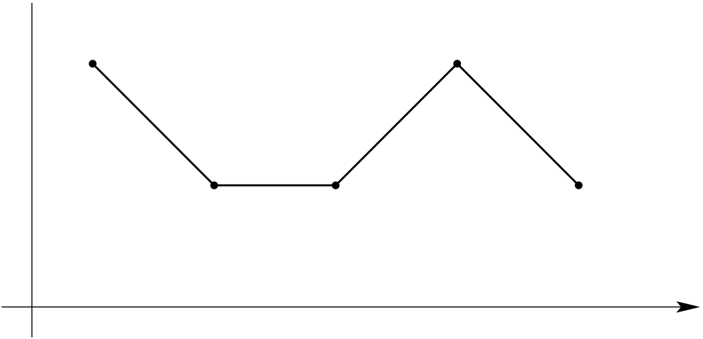
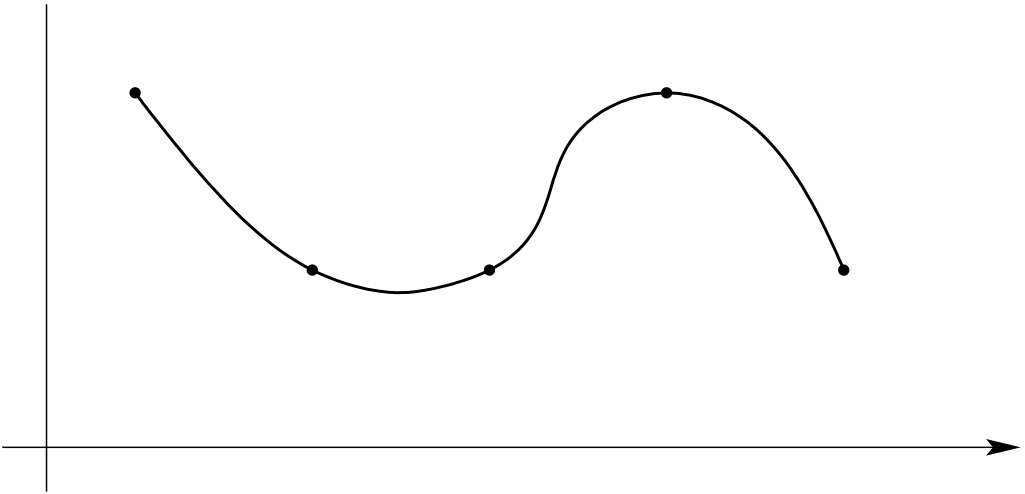
Of particular interest will be the cubic spline interpolation. For cubic splines, we will build our interpolant using piecewise cubic polynomials. At the sub-interval interfaces, we will require continuity of the interpolant and its derivative up to the second order. In this way, we can combine our goal of reducing over-/under-shooting with a smooth-looking interpolant.
10.1 Piecewise Linear Interpolation
We start by recalling the ideas for piecewise linear interpolation from Chapter 6. In Section 6.7, we have used linear functions on the sub-intervals of \([x_i,x_{i+1}]\subseteq [a,b],\) leading to the space of continuous and piecewise linear functions on \([a,b]\) \[U_n \;=\; S_n \;=\; \left\{v \;|\; v \in C([a,b]), \; v|_{[x_{k-1},x_k]} \in P_1, \, k = 1,\ldots, n\right\}\, .\]
The interpolation problem \[u_n \in S_n:\;u_n(x_k)\;=\;f(x_k),\qquad k=0,\ldots, n\] has solution \[\begin{aligned} u_n \;&=\; \sum_{k=0}^n f(x_k) \varphi_k\\ \text{with } \varphi_k\in S_n \text{ fulfilling } \varphi_k (x_l) \;&=\; \delta_{kl}\, , \end{aligned}\] the so-called nodal basis.
We would like to investigate this construction in more detail
on each sub-interval \([x_{k-1},x_k]\) we took polynomials of first order for building the interpolant. In principle, with \(2\) degrees of freedom per sub-interval, we would have in total \(2n\) degrees of freedom.
the polynomials on the sub-intervals were “glued” together by the condition \(v \in C([a,b]),\) i.e. by requiring global continuity. This condition removes one degree of freedom at each interface, leading to \(2n-(n-1)=n+1\) remaining degrees of freedom.
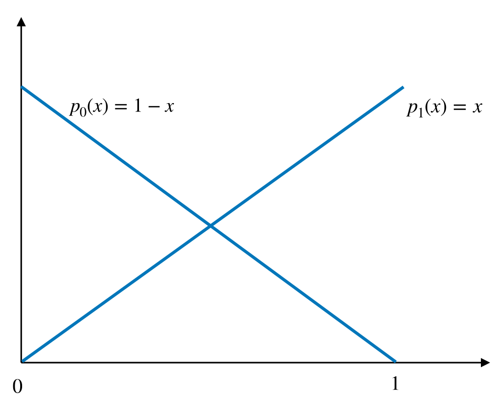
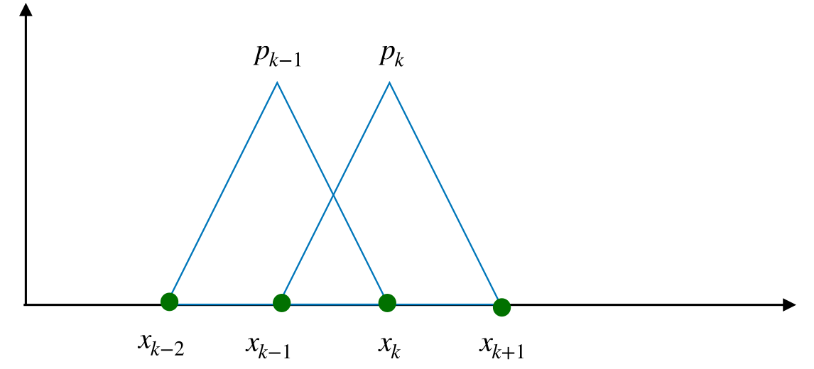
Our interpolant was eventually expressed as a linear combination of the nodal basis functions (hat functions). The hat function at point \(x_k\) can be constructed as the sum of two Lagrangian basis functions of \(P_1([x_{k-1},x_k])\) and \(P_1([x_{k},x_k+1]),\) respectively.
Figure 10.2 illustrates this connection process: two Lagrangian basis functions (left picture) get connected, such that the resulting (hat) function (right picture) is continuous. We call the hat functions also nodal basis functions.
10.2 Cubic Spline Interpolation
The motivation to define the cubic spline interpolation is the increase of the global smoothness of the interpolating function. In this context, the “smoothness” of the interpolant \(\phi\) can be interpreted as cumulative curvature.
Let \(\Delta=\{ a=x_0<x_1<\cdots<x_n=b\}\) be a set of nodes. We set \(I_k=[x_{k},x_{k+1}]\) and \(h_k=x_{k+1}-x_{k},\) \(k=0, \ldots, n-1.\) We now incorporate the smooth transition at the borders between the sub-intervals into our problem formulation.
We will denote by \(C^{m}([a,b])\) the space of all functions with \(m\) continuous derivatives on the interval \([a,b].\)
Definition 10.1 • Cubic splines
The spline functions of order \(m\) for the mesh \(\Delta\) are defined by \[S_{\Delta}^m \;=\; \left\{ v \in C^{m-1}([a,b]),\; v|_{I_k} = S_k \in P^m\right\}.\] The case \(m=3\) is called cubic splines.
We now consider the interpolation problem \[\tag{10.1} s\in S_{\Delta}^m:\;s(x_k) \;=\; f(x_k)\qquad \forall k=0,\ldots, n.\]
Each \(v\in S_{\Delta}^m\) is determined by \(n\) polynomials \(S_k,\) \(k=0,\ldots, n-1\) of order \(m,\) leading to a total of \(n \cdot (m+1)\) coefficients. The requirement \(v\in C^{m-1}\) gives rise to \(m \cdot (n-1)\) interface conditions: \[S_k^{(j)}(x_{k+1}) \;=\; S_{k+1}^{(j)}(x_{k+1}),\qquad j=0, \ldots, m-1,\;k = 0, \ldots, n-2\]
The resulting equations for the coefficients of the local polynomials \(S_k,\) \(k=0, \ldots, n-1\) can be shown to be linearly independent which here, however, we do not show. Thus, we get \[\dim S_{\Delta}^m \;=\; n(m+1)-(n-1)m \;=\; n+m\] We have \(n+1\) interpolation conditions from (10.1). Since we have \[\dim S_{\Delta}^m-(n+1) \;=\; m-1,\] we have to prescribe additional \(m-1\) conditions.
For the case \(m=1\) we have \(m-1=0,\) so no additional conditions have to be imposed. However, for the case \(m=3\) (cubic splines) we need \(m-1=2\) additional conditions. This is normally done via boundary conditions at \(a\) and \(b.\) The most commonly used ones are
natural boundary conditions: \(s^{\prime\prime}(a) = s^{\prime\prime}(b) = 0.\)
prescribed boundary derivatives: \(s^\prime(a) = f_0^\prime\) and \(s^\prime(b) = f_n^\prime,\) where \(f_0^\prime\) and \(f_n^\prime\) are prescribed values of either the function’s actual derivative or an approximation thereof.
periodic boundary conditions: \(s(a) = s(b)\) and \(s^\prime(a) = s^\prime(b).\)
10.3 A Mechanical Motivation
The content of this subsection is for motivational purposes and can be ignored on first reading. The following arguments explain why the name “spline” has been chosen.
Definition 10.2 • Mean curvature
Consider a spline \[\psi \in C_{\Delta}^2([a,b]) \;=\; \left\{ v \in C^2([a,b]),\; v(x_k) = f(x_k), k = 0,\ldots, n \right\}\] described by the nodes \((x_k, f(x_k))\) with prescribed boundary derivatives. The mean curvature of \(\psi\) is defined by \[{\mathcal K}(x) \;=\; \frac{\psi^{\prime\prime}(x)}{(1+\psi^\prime(x)^2)^{3/2}}\]
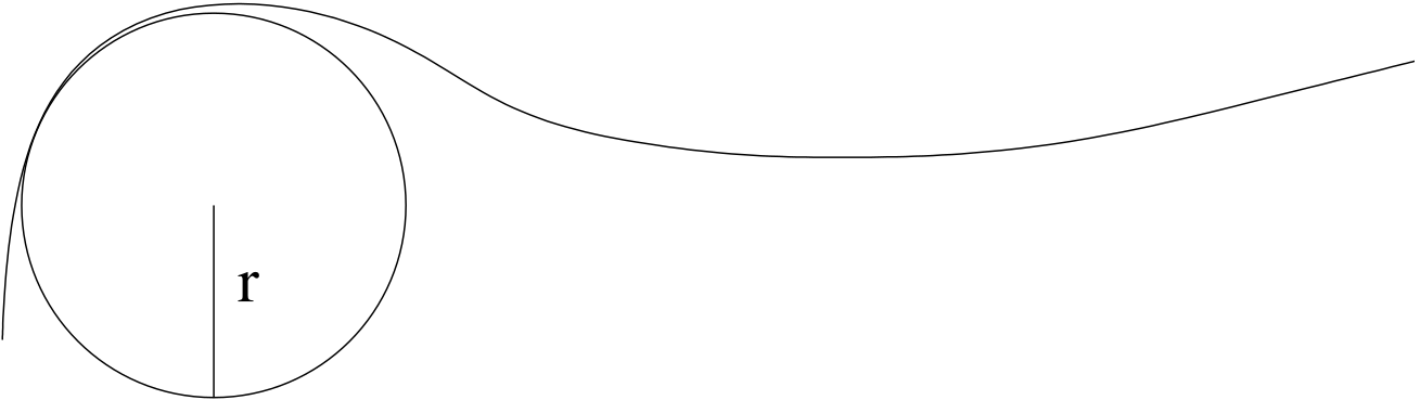
Curvature can also be interpreted as the radius \(r\) of an osculating circle, cf. Figure 10.3 by the relation \(|{\mathcal K}(x)| = \frac{1}{r}.\)
For small displacements, we have \({\mathcal K}(x) \approx \psi^{\prime\prime}(x)\) and we can measure the elastic energy or bending energy of the spline by means of \[E(\psi) \;=\; \int_a^b \, (\psi^{\prime\prime})^2 \, \approx \int_a^b \, ({\mathcal K}(x))^2 \, dx.\] The elastic energy \(E\) should be minimal on the set of all possible configurations of the spline, which fulfill the natural boundary conditions. Technically, this means that we are looking for a function \(\psi\) in the set \[H \;=\; \left\{ v \in C_{\Delta}^2([a,b]),\; v^{\prime}(a) = f^{\prime}(a),\; v^{\prime}(b) = f^{\prime}(b)\right\}\,\] which has minimal elastic energy \(E(\psi).\) Setting \(\|v\|_{L^2}^2 := \int_a^b \, v^2 \, dx,\) we thus get the minimization problem \[\text{Find } \psi \in H: \; \left\|\psi^{\prime\prime}\right\|_{L^2} \;\leq\; \left\|v^{\prime\prime}\right\|_{L^2} \qquad \forall v \in H.\]
Theorem 10.1
Let \(s \in S_{\Delta}^3\) be the solution of the interpolation problem (10.1) and let \(v \in C_{\Delta}^2([a,b]).\) Then, if \[\tag{10.2} s^{\prime\prime}(x) \left.\left(v^{\prime}(x)-s^{\prime}(x)\right) \right\rvert_a^b \;=\; 0\] we get the estimate \[\tag{10.3} \left\|s^{\prime\prime}\right\|_{L^2} \;\leq\; \left\|v^{\prime\prime}\right\|_{L^2}\]
Remark 10.1
The above theorem states nothing less than that the spline interpolation is the function with the smallest second derivative that fulfills the interpolation conditions. Thus, it avoids over- and under-shooting.
10.4 Computing a cubic spline
Up to now, we have just looked at splines from a purely theoretical point of view. We have stated neither a precise expression for one nor a way to compute its coefficients. The spline \(s\in S_\Delta^n\) is actually made up of \(n\) separate parts \(S_i,\) \(0\leq i\leq n-1,\) which are defined on \([x_i,x_{i+1}].\) These are cubic polynomials.
First, let us assume we have a set of nodes \(x_0 < x_1 < \ldots < x_n\) with \(x_i\in[a,b],\) \(x_0=a\) and \(x_n=b.\) We define their differences \(h_i\) by \(h_i = x_{i+1} - x_i.\) We can now write the \(S_i\) as follows: \[\begin{aligned} S_i(x) \;=\quad a_i + b_i(x-x_i)+\frac{c_i}{2}(x-x_i)^2+\frac{d_i}{6}(x-x_i)^3 \end{aligned}\] We now need to take care of the transition condition between the sub-intervals. This is a good exercise in bookkeeping.
10.4.0.0.1 Continuity and Interpolation Conditions
We get \(2n\) conditions, since for \(i=0,\ldots,n-1\) it holds \[\begin{aligned} S_i(x_i)=y_i \end{aligned}\] Leading to \[\tag{10.4} \begin{aligned} S_i(x_i) &= y_i = a_i \qquad\text{left end-point}\\ S_i(x_{i+1}) &= y_{i+1} = a_i+b_i h_i +\frac{c_i}{2} h_i^2 +\frac{d_i}{6}h_i^3 \qquad\text{right end-point} \end{aligned}\]
10.4.0.0.2 Continuity of the First Derivative
We get \(n-1\) conditions, since for \(i=0,\ldots,n-2\) it holds at the inner points \[\tag{10.5} \begin{aligned} S_i'(x_{i+1}) &= S_{i+1}'(x_{i+1}) = b_i + c_i h_i +\frac{d_i}{2} h_i^2 = b _{i+1} \end{aligned}\]
10.4.0.0.3 Continuity of the Second Derivative
We get \(n-1\) conditions, since for \(i=0,\ldots,n-2\) it holds at the inner points \[\tag{10.6} \begin{aligned} S_i''(x_{i+1}) &= S_{i+1}''(x_{i+1}) = c_i + d_i h_i = c_{i+1} \end{aligned}\]
10.4.0.0.4 Boundary Conditions
We get \(2\) conditions, at the boundary points from the boundary conditions. Here, we took natural boundary conditions. \[\begin{aligned} S_0''(x_0) &= 0 = c_0\\ S_{n-1}''(x_n) &= 0 = c_{n-1}+d_{n-1}h_{n-1} \end{aligned}\] We then use (10.6) and (10.4) to define \(d_i\) and \(b_i\) respectively and substitute them into (10.5). This leads to the following equation for \(i=0,\ldots,n-2\) \[\tag{10.7} h_ic_i+2(h_{i+1}+h_i)c_{i+1} + h_{i+1}c_{i+2} = 6\left(\frac{y_{i+2}-y_{i+1}}{h_{i+1}} - \frac{y_{i+1}-y_{i}}{h_{i}} \right)\, .\] For the ease of notation, we have set \(c_n=0.\)
For equidistant nodes with \(h_i=h\) we get \[hc_i+4hc_{i+1}+hc_{i+2} = \frac{6}{h}(y_{i+2}-2y_{i+1}+y_i)\] which we can write with \(k=i+1\) for easier indexing as \[hc_{k-1}+4hc_{k}+hc_{k+1} = \frac{6}{h}(y_{k+1}-2y_{k}+y_{k-1})\, .\] The resulting linear system then is tri-diagonal and can be solved with, e.g. Gaussian elimination, for the coefficients \(c_i.\) The remaining coefficients \(a_i,d_i,b_i\) can then be computed for \(i=0,\ldots,n-1\) with the elementary formulas \[\begin{aligned} a_i&=y_i\\ d_i &= \frac{c_{i+1}-c_i}{h_i}\\ b_i&= \frac{y_{i+1}-y_i}{h_i} - \frac{1}{2}c_ih_i-\frac{1}{6}d_ih_i^2 \end{aligned}\] For example, for an equidistant mesh, we would get for the coefficient matrix \(H\) from (10.7) \[H \;=\; \begin{pmatrix} 4h & h \\ h & 4h & & h && 0 \\ 0 & h & & 4h && h && 0 \\ & & \ddots & & \ddots & & \ddots \\ & 0 && h && 4h && h \\ & && & & h && 4h \end{pmatrix}\] AXXBT4G1LW49PVMSAKZCQJVITZOSNORP
11 Least Square Problems and the Normal Equations
11.1 General Setting and Choice of the Approximation
In this chapter, we consider the problem of parameter identification from measured data. Our presentation follows —in a reduced way— the chapter on Least Square problems in Hohmann, Andreas, and Peter Deuflhard. Numerical analysis in modern scientific computing: an introduction. Vol. 43. Springer Science and Business Media, 2003.
We assume that we have \(m\) pairs of measured data \[(t_i,b_i), \;\;\; t_i,b_i\in\mathbb{R}\, \qquad i=1,\ldots,m\, ,\] available. We assume that there is a mapping \(\varphi\colon\mathbb{R}\longrightarrow\mathbb{R},\) such that \[b_i\approx \varphi(t_i)\, \qquad i=1,\ldots,m\, ,\] where the \(b_i\) are interpreted to be perturbed data, e.g. by measurements.
We now would like to find an approximation \({\mathcal N}\colon \mathbb{R}\longrightarrow\mathbb{R}\) to \(\varphi,\) which shall depend on the parameter vector \(x\in\mathbb{R}^n,\) i.e. \[{\mathcal N}(t;x) \approx \varphi(t)\, .\] Obviously, the mapping \(\varphi\) in general can be of arbitrary form. In order to simplify the construction of our model \({\mathcal N}(t;x) ,\) we therefore assume that the model \({\mathcal N}(\cdot;x)\) will depend linearly on the parameters \(x_1,\ldots,x_n\in\mathbb{R}.\) We therefore make the following Ansatz \[\tag{11.1} {\mathcal N}(t;x) = x_1 \cdot a_1(t)+\ldots+ x_n \cdot a_n(t)\] with \(a_i\colon\mathbb{R}\longrightarrow\mathbb{R},\) \(i=1,\ldots,n\) arbitrary functions. Here, we assume that the \(a_i\) are continuous. The choice of the functions \(a_i\) determines implicitly which functions we can approximate well. For example, if we would know that \(\varphi\) is a linear function, i.e. \(\varphi(t)=c_1 +c_2t,\) with \(c_1,c_2\in\mathbb{R}\) arbitrary but fixed, we could choose \(a_1 \equiv 1\) and \(a_2(t)=t.\) Then, \({\mathcal N}(t;x) = x_1 \cdot a_1(t) +x_2 \cdot a_2(t) = x_1 + x_2t\) and we would expect that for the solution \((x_1,x_2)^T\) of the least square system we would have \((x_1,x_2)\approx (c_1,c_2).\) However, in general, \(\varphi\) is unknown and we cannot expect that \(\varphi \in \mathrm{span}\{a_1,\ldots,a_n\}\) as it was the case in our simple example above.
11.2 Least Squares
We now discretize our Ansatz functions \(a_i\) by taking their values at the points \(t_i\) and set \[\tag{11.2} a_{ij} = a_j(t_i)\, \qquad i=1,\ldots,m,\quad j=1,\ldots,n\, .\] Setting \(A=(a_{ij})_{i=1,\ldots,m,\, j=1,\ldots,n}\) and \(b=(b_1,\ldots, b_m)^T,\) we end up with the linear system (\(m>n\)) \[Ax=b\, .\] Here and in the following we will always assume that \(A\) has full rank, i.e. \(\mathrm{rank}(A)=n.\) Since \(A\) cannot be inverted, we decide to minimize the error of our approximation \(Ax\) to \(b.\) More precisely, we see that \[{\mathcal N}(t_i; x) = \sum_{j=1}^n x_j \cdot a_j(t_i) = (Ax)_i\, ,\] and therefore decide to minimize the error \[\tag{11.3} \min_{x\in\mathbb{R}^n} \|Ax-b\|\] of our approximation in a suitable norm \(\|\cdot \|.\) The choice \(\|\cdot\|=\|\cdot\|_2\) leads to \[\|Ax-b\|_2^2 = \sum_{i=1}^m ({\mathcal N}(t_i; x) - b_i)^2 = \sum_{i=1}^m \Delta_i^2 \, ,\] where we have set \(\Delta_i = {\mathcal N}(t_i; x) - b_i.\) Thus, minimizing the error \(\|Ax-b\|_2\) in the Euclidean norm corresponds to minimizing the (sum of the) squared errors \(\Delta_i.\) This motivates the name least squares.
11.3 Normal Equations
Fortunately, the solution of the minimization problem (11.3) can be computed conveniently by solving the so-called normal equations \[\tag{11.4} A^TAx=A^Tb\, .\] We recall that in this chapter we always assume that \(A\) has full rank, i.e. \(\text{rank}(A)=n.\) The derivation of the normal equations (11.4) is closely connected to the concept of orthogonality.
We start our considerations by investigating the set of possible approximations, which is given by the range of \(A\) \[\tag{11.5} R(A) = \{y\,|\,y\in \mathbb{R}^m, y=Ax\}\, .\] We note that from the definition of the matrix-vector multiplication (7.15) that \(R(A)\) is the linear space spanned by the columns of \(A,\) i.e. \[R(A) = \mathrm{span} \{A^1,\ldots,A^n\}\,,\] and we can write the elements \(y\in R(A)\) as linear combinations of the columns of \(A\) \[y\in R(A) \Leftrightarrow y = \sum\limits_{i=1}^n \alpha_i A^i\, ,\qquad \alpha_1,\ldots,\alpha_n\in \mathbb{R}\, .\]
As a candidate for the solution \(x\) of the minimization problem (11.3), with \(\|\cdot\|=\|\cdot\|_2,\) we take the element \(x\in R(A)\) which is characterized by the fact that the corresponding error \(b-Ax\) is orthogonal to \(R(A)\): \[\tag{11.6} \begin{aligned} & \langle Ax-b, y\rangle = 0 \qquad \forall y \in R(A)\\ \Leftrightarrow\quad & \langle Ax-b, Az\rangle = 0 \qquad \forall z \in \mathbb{R}^n\\ \Leftrightarrow\quad & \langle A^T(Ax-b), z\rangle = 0 \qquad \forall z \in \mathbb{R}^n\\ \Leftrightarrow\quad & A^T(Ax-b) = 0 \\ \Leftrightarrow\quad & A^TAx = A^Tb \, . \end{aligned}\] The fact that the error \(b-Ax\) is orthogonal to \(R(A)\) induces also a best approximation property of \(Ax\) of the normal equations (11.4) in the Euclidean norm.
Theorem 11.1
Let \(m>n\) and let \(A\in\mathbb{R}^{m \times n}\) have full rank. Let furthermore \(b\in\mathbb{R}^m\) be given. Then, for the solution \(x\) of the normal equations \(A^T Ax=A^Tb,\) we have the following best approximation property for \(Ax\) in the Euclidean norm \[\tag{11.7} \|Ax-b\|_2 = \min_{z\in R(A)} \|z-b\|_2\, .\]
Proof. We have for \(z\in R(A)\) \[\begin{aligned} \|z - b\|_2^2 & = \|z - Ax + Ax - b\|_2^2\\ & = \|z - Ax\|_2^2 + 2 \langle z-Ax, Ax-b\rangle + \|Ax - b\|_2^2 \\ & = \|z - Ax\|_2^2 + \|Ax - b\|_2^2 \\ & \geq \|Ax - b\|_2^2 \, . \end{aligned}\] Here, we have exploited that, due to \(z-Ax\in R(A)\) and the orthogonality condition (11.6), we have \(\langle z-Ax, Ax-b \rangle = 0.\)
Proof. Exercise.
For later reference, we rewrite this result in a more abstract form
Corollary 11.2
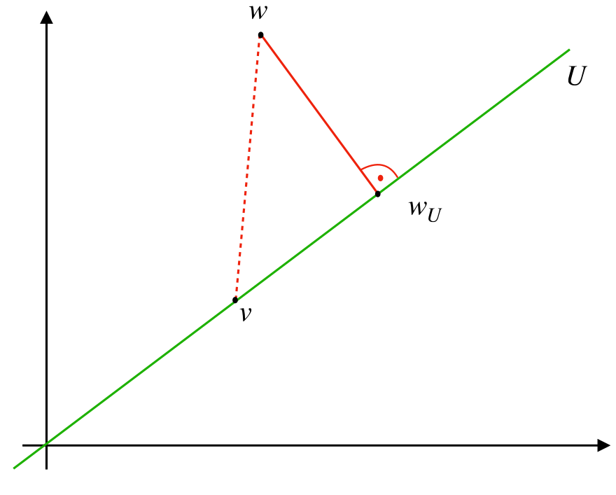
Let \(m\geq n\) and let \(U=\mathrm{span}\{u_1,\ldots,u_n\}\subset \mathbb{R}^m.\) Let furthermore \(w\in\mathbb{R}^m\) and let \(w_U\) be the unique element in \(U\) with \(w - w_U \bot U,\) i.e. \(\langle w-w_U, v\rangle = 0\) for all \(v\in U.\) Then we have \[\tag{11.8} \|w-w_U\|_2 = \min_{v\in U} \|w-v\|_2\, .\]
The proof is literally taken from the above theorem. We repeat it here for notational convenience.
Proof. We have for \(v\in U\) \[\begin{aligned} \|w - v\|_2^2 & = \|w - w_U + w_U - v\|_2^2\\ & = \|w - w_U\|_2^2 + 2 \langle w - w_U, w_U - v\rangle + \| w_U - v\|_2^2 \\ & = \|w - w_U\|_2^2 + \|w_U - v\|_2^2 \\ & \geq \|w - w_U\|_2^2 \, . \end{aligned}\]
We call \(w_U\) the orthogonal projection of \(w\) into \(U\) and refer to Figure 11.1 for a graphical representation.
11.3.0.0.1 Pseudo-Inverse
If \(A\) has full rank, the solution \(x\) of the normal equations (11.4) can be formally written as \[x = (A^TA)^{-1}A^Tb\, .\] This gives rise to the definition of the pseudo-inverse \(A^+\) of \(A\) as \[\tag{11.10} A^+ = (A^TA)^{-1}A^T \, .\] From the definition, we see that \(A^+A = (A^TA)^{-1}A^TA = I_n,\) if \(A\) has full rank. This motivates the name pseudo-inverse.
11.4 Condition Number of the Normal Equations
A straightforward approach for solving the normal equations (11.4) would be to compute \(A^TA\) and \(A^Tb\) and then to apply Cholesky decomposition to the resulting linear system. Although this can be done, in many cases it might not be advisable. The main reason is the condition number of \(A^TA.\)
We recall for our investigations on \(\kappa(A^TA)\) the condition number of a rectangular matrix (8.7), which was defined as \[\kappa(A) = \frac{\max_{\|x\| = 1} \|Ax\|}{\min_{\|x\|=1} \|Ax\|}\, .\] Before proceeding, we show that this definition is compatible with our definition (8.6) for invertible matrices. We first note that the numerator, by definition, is the norm \(\|A\|\) of \(A.\) We continue by investigating the denominator and assume that \(A\in \mathbb{R}^{n \times n}\) and that \(A^{-1}\) exists. Then, we have \[\begin{aligned} \frac{1}{\min\limits_{\substack{\|x\|=1 \\ x\in\mathbb{R}^n}} \|Ax\|} & = \frac{1}{\min\limits_{0\not = x\in\mathbb{R}^n} \frac{\|Ax\|}{\|x\|}}\\ & = \max\limits_{0\not = x\in\mathbb{R}^n}\frac{1}{\frac{\|Ax\|}{\|x\|}}\\ &= \max\limits_{\substack{0\not = y\in\mathbb{R}^n \\ y=Ax}}\frac{\|A^{-1}y\|}{\|y\|}\\ & =\|A^{-1}\|\\ \end{aligned}\] Putting everything together, we see that for invertible \(A\) we have \[\kappa(A) = \frac{\max_{\|x\| = 1} \|Ax\|}{\min_{\|x\|=1} \|Ax\|} = \|A\| \cdot \|A^{-1}\|\, .\] It now can be shown that the condition number of \(A^TA\) is the square of the condition number of \(A,\) i.e. \[\tag{11.11} \kappa(A^TA) = (\kappa(A))^2\, .\] Thus, in general, it is not advisable to set up \(A^TA\) for solving the normal equations. Instead, as we will see later in the lecture on numerical methods, we will use the so-called \(QR\)-decomposition. The \(QR\)-decomposition is a relative of the \(LU\)-decomposition, which uses orthogonal transformations as elementary transformations.