7 Polynomial Interpolation
7.1 Interpolation Conditions
One of the most fundamental techniques in computational science is interpolation: Given a set of points \(x_i\in\mathbb{R}\) and a set of corresponding data \(y_i \in \mathbb{R},\) \(i=0,\ldots, n,\) we look for a function \(f\colon\mathbb{R}\longrightarrow \mathbb{R}\) such that the interpolation conditions \[\tag{7.1} f(x_i) = y_i,\qquad i=0, \ldots, n\] are fulfilled. Obviously, the conditions (7.1) prescribe the values of \(f\) only at the points \(x_i.\)
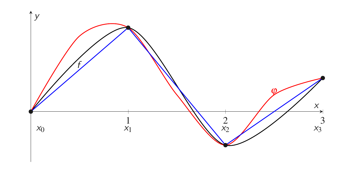
Some examples can be found in Figure 7.1.
From a general point of view, we are interested in a method which
has a small approximation error on our interval of interest \([a,b],\) i.e. we can control and bound the quantity \[\tag{7.2} \begin{aligned} \mathrm{err}_f(\varphi) = \sup_{x\in[a,b]} |f(x) - \varphi(x)| =: \|f-\varphi\|_\infty \end{aligned}\]
is robust in the sense that small changes in the input do lead to small changes in the output only, i.e. a bounded condition number of the mapping \(f\mapsto \varphi,\)
provides a low complexity of the respective algorithms for computing and evaluating \(\varphi.\)
The interpolation can be regarded as a “reconstruction problem”: given the \(n+1\) values \(f(x_0),\ldots,f(x_n)\) of a function \(f\) at the points \(x_0,\ldots, x_n,\) which form our mesh \(\Delta_n,\) \[\tag{7.3} \Delta_n \;=\; \left\{ x_0, \ldots, x_n \;|\; a \leq x_0 < x_1 < \cdots < x_n \leq b\right\} \subset [a,b]\, ,\] we aim to reconstruct \(f\) with the highest possible accuracy. Here, we only will consider continuous functions, i.e. functions which do not “jump” or do not have “holes” in their graph. For convenience, we will denote the set of all continuous and real-valued functions on the interval \([a,b]\) by \(C([a,b])\)
Our goal is to construct a function \(\varphi\in C([a,b]),\) which is intended to approximate \(f\) as well as possible. The minimal requirement we have is that \(\varphi\) fulfills the so-called interpolation conditions \[\tag{7.4} \varphi(x_i) = f(x_i)\, , \qquad i = 0, \ldots, n\, .\]
As can be seen in Figure 7.1, \(\varphi\) can be chosen in many different ways. Widely used methods for constructing approximations \(\varphi\) include
polynomial interpolation
piecewise polynomial interpolation
(B-)splines
trigonometric interpolation
These methods above have some common structure. The function \(\varphi\) should be “easy to handle” so that we can plot it, differentiate it, or integrate it without significant problems.
A typical choice is to use polynomials, i.e. to look for our interpolant \(\varphi\) in the space of all polynomials of degree \(n\): \[\varphi \in P^n([a,b]) =\{p \,|\, p\colon [a,b]\longrightarrow \mathbb{R},\, p(x) = \sum_{i=0}^n a_ix^i\,, \, a_0,\ldots,a_n\in\mathbb{R}\}\, .\] Here, we have decided to use \(P^n([a,b])\) as our “approximation space”. We also note that choices other than polynomials are possible, such as trigonometric functions, exponential functions, rational functions, etc. Here, we focus on polynomials as they are most widely used for building approximation spaces.
We note that from now on we will often write \(P^n\) instead of \(P^n([a,b])\) in order to simplify the notation.
We are especially interested in the question of whether for a given \(f\) there exists a unique \(p_n\in P^n\) which fulfills the interpolation conditions (7.4), \[p_n(x_i) \;=\; f(x_i),\qquad i = 0, \ldots, n\]
As pointed out above, the idea of polynomial interpolation is to construct the sought-after approximation \(\varphi\) as a polynomial of degree less or equal to \(n,\) i.e. we assume that \(\varphi\) has the form \[\tag{7.5} \varphi (x) = a_nx^n+\cdots + a_1 x + a_0 = \sum\limits_{i=0}^{n} a_ix^i\, .\] where \(a_0,\ldots,a_n \in \mathbb{R}\) are the coefficients of the polynomial. In Equation (7.5), \(\varphi\) is given with respect to the monomial basis \(\{1,x,x^2,x^3,\ldots,x^n\}.\) As we will see later, also different representations of \(\varphi,\) which do not use monomials, are possible. Thus, it is important to distinguish between the polynomial \(\varphi\) and its representations.
In \(P^n([a,b]),\) the interpolation problem reads:
Given \(f \in C([a,b]),\) find for a given grid \(\Delta_n\) a function \(p_n\in P^n\) with \[\tag{7.6} p_n(x_i) = f(x_i), \qquad i=0, \ldots, n\, .\]
We would like to understand whether the interpolant exists and is unique. We start with uniqueness.
Theorem 7.1 • Uniqueness of the Interpolation Polynomial
If the interpolation problem (7.6) has a solution, it is unique.
Proof. Let \(p, q\in P^n\) be two interpolation polynomials with \(p(x_i)=q(x_i) = f(x_i)\) for \(i=0,\ldots, n.\) Then, \(p-q\) is a polynomial of degree less than or equal to \(n\) with the \(n+1\) zeros \(x_0,\ldots,x_n.\) Since a non-constant polynomial of degree \(n\) can have at most \(n\) zeros, \(p-q\) has to be the null polynomial.
Note 7.1
We supposed that all \(x_i\) are distinct. Otherwise, we would have less than \(n+1\) zeros of \(p-q.\)
We will show the existence of the interpolation polynomial later using Lagrange polynomials.
Due to the uniqueness proved in 7.1, we can write the solution to the interpolation problem (7.6) as \(p_n=p(x_0, \ldots, x_n|f).\) As an additional simplification, we consider the affine transformation \[\eta=\eta(x)=a+x\cdot (b-a)\, .\] It translates and rescales the interval \([0,1]\) to \([a,b].\) Therefore, it suffices to consider (7.6) on the fixed interval \([0,1]\) from now on.
There are several ways to represent the polynomials in \(P^n.\) Two of the most common are
the monomes \(x^i,\; i=0, \ldots, n\) and
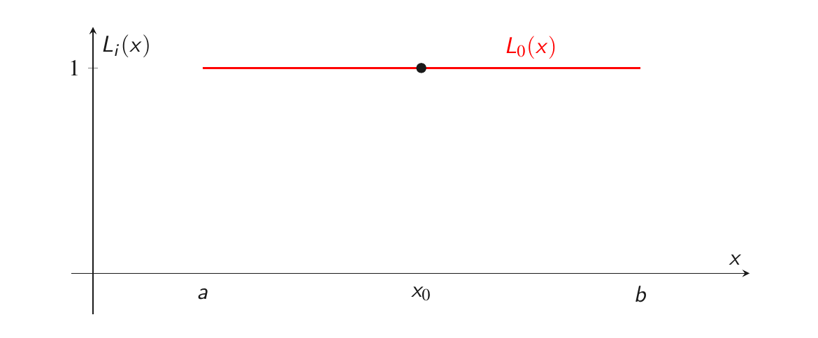
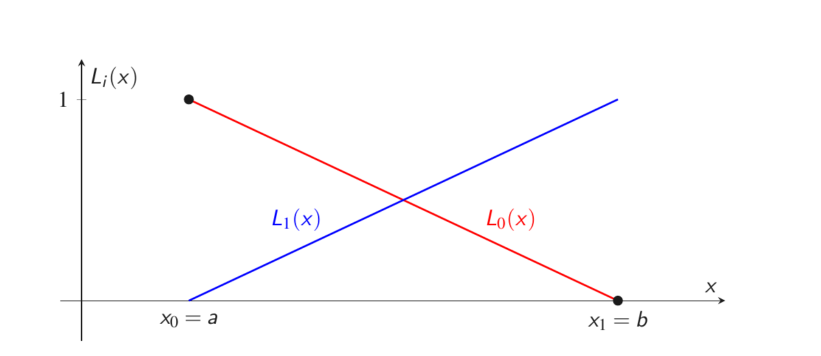
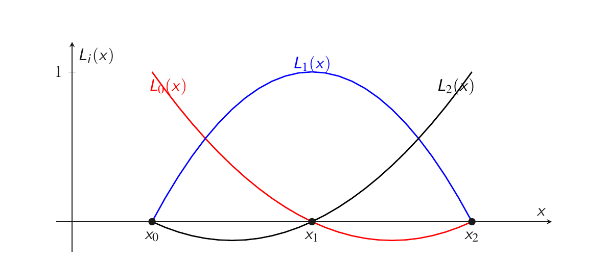
the Lagrangian polynomials \(L_k^n,\) sometimes called the nodal basis with \(L_i^n(x_j)=\delta_{ij}\) for \(x_j\in\Delta_n.\)
Here, we have used the Kronecker-\(\delta\) \[\tag{7.7} \begin{aligned} \delta_{ij} =\left\{\begin{aligned}1 &, \, i=j\\ 0 &,\, i\not= j\end{aligned}\right. \end{aligned}\] The Lagrangian basis functions can be written as \[\tag{7.8} L_i^n(x)\;=\;\prod_{\substack{k=0\\k \neq i}}^n\, \frac{x-x_k}{x_i-x_k},\qquad i=0, \ldots, n.\] In particular, we have that \[\tag{7.9} p_n(x) = p(x_0, \ldots, x_n|f) \;=\; \sum_{i=0}^n f(x_i)L_i^n(x)\, .\] Please note that in Equation (7.9) the values \(f(x_i)\) are the coefficients of \(p_n\) with respect to the Lagrangian basis.
Remark 7.1
We can define by means of the Euclidean scalar product \(\langle \cdot,\cdot \rangle\) a scalar product on \(P^n\) as follows: \[\tag{7.10} \langle p,q \rangle \;=\; \sum_{i=0}^n p(x_i)\cdot q(x_i)\, .\] Inserting \(p=L_k^n\) and \(q=L_l^n\) into Equation (7.10), we get \[\begin{aligned} \langle L_k, L_l\rangle \;&=\; \sum_{i=0}^n L_k(x_i)L_l(x_i)\\ &=\; \sum_{i=0}^n \delta_{ki}\delta_{li} \;=\; \delta_{kl}, \, \end{aligned}\] which implies that the Lagrange polynomials are orthogonal with respect to the scalar product (7.10).
In Figure 7.2–Figure 7.4, the Lagrangian polynomials are plotted for \(n=0,1,2.\)
Remark 7.2
Computing the coefficients \(\{a_i\}\) of \(p_n\) with respect to the monomial basis leads to the following system of linear equations: \[\underbrace{\begin{pmatrix} 1 & x_0 & x_0^2 & \cdots & x_0^n\\ \vdots & \vdots & \vdots & & \vdots\\ 1 & x_n & x_n^2 & \cdots & x_n^n \end{pmatrix}}_{=:\;{\mathcal V}_n} \begin{pmatrix} a_0\\ \vdots\\ a_n \end{pmatrix} \;=\; \begin{pmatrix} f(x_0)\\ \vdots \\ f(x_n) \end{pmatrix} \tag{7.11}\] The matrix \({\mathcal V}_n\) is called the Vandermonde Matrix . Its determinant can be computed as follows: \[\det({\mathcal V}_n) \;=\; \prod_{i=0}^n \, \prod_{j=i+1}^n(x_i-x_j).\] It is different from \(0\) if all \(x_i\) are distinct. For large \(n,\) the Vandermonde matrix \({\mathcal V}_n\) becomes almost singular. This means that we have to solve a badly-conditioned system. Furthermore, the solution of this system also might require a substantial amount of time, i.e. it is of order \(O(n^3),\) as the matrix \({\mathcal V}_n\) is dense. We want to avoid this and, therefore, look for alternative ways to compute and evaluate the interpolation polynomial.
The particular form of the Lagrange polynomials allows us to provide an existence result for our interpolation problem.
Theorem 7.2 • Existence of the Interpolation Polynomial
The interpolation problem (7.6) has a solution in \(P^n.\)
Proof. Set \[\varphi(x) = \sum_{i=0}^n f(x_i) L_i^n (x)\, .\] We have \(\varphi\in P^n.\) Furthermore, we have for \(i=0,\ldots,n\) that \[\varphi(x_j) = \sum_{i=0}^n f(x_i) L_i^n (x_j) = \sum_{i=0}^n f(x_i) \delta_{ij} = f(x_j)\, .\] Thus, \(\varphi\) fulfills the interpolation conditions (7.1).
Together with Theorem 7.2, we therefore have shown:
Corollary 7.3
The interpolation problem (7.6) has a unique solution in \(P^n.\)
We note that also other interpolants can be constructed. Our existence and uniqueness result has been shown only for polynomials of order \(n,\) i.e. for \(P^n\) as the approximation space. Furthermore, the interpolation polynomial in general will depend on the chosen mesh \(\Delta_n.\)
7.2 Properties of the Interpolation Process
Since the interpolation problem (7.1) has a unique solution in \(P^n,\) it is justified to think about interpolation as a mapping from “data space” to “polynomial space”. As we can see from (7.1), the interpolation polynomial is constructed by taking the values of \(f\) at the mesh points \(x_0,\ldots,x_n\) and then building the interpolation polynomial using (7.9). Thus, as “data space” we can identify the space of continuous functions \(C([0,1]),\) and the function \(f\in C([0,1])\) is our input. The output of our interpolation mapping then is simply the interpolation polynomial \(p(x_0,\ldots,x_n|f).\)
The above considerations motivate us to make the following definition.
Definition 7.1 • Interpolation operator
We call the mapping \[\tag{7.12} \begin{aligned} I _n:\; C([0,1]) \;&\longrightarrow\; P^n([0,1])\\ f \;&\longmapsto\; p_n = p(x_0,\ldots, x_n|f) \end{aligned}\] interpolation operator and we write \[I_n(f) = p(x_0,\ldots, x_n|f) = p_n\, .\]
We would like to collect some properties of the interpolation operator or, in other words, we would like to understand the process of interpolation better.
Our first question is connected to the question of what will happen if we multiply the function \(f\) by a scalar \(\alpha \in\mathbb{R},\) i.e. how are the two polynomials \(p(x_0,\ldots, x_n|f)=I_n(f)\) and \(p(x_0,\ldots, x_n|\alpha f)=I_n(\alpha f).\) related? We answer this question by computing \[\begin{aligned} I_n(\alpha f) & = p(x_0,\ldots, x_n|\alpha f) \\ & = \sum_{i=0}^n \alpha \cdot f(x_i) L_i^n\\ & = \alpha \sum_{i=0}^n f(x_i) L_i^n\\ &= \alpha \cdot p(x_0,\ldots, x_n|f) \\ &= \alpha \cdot I_n(f)\, . \end{aligned}\] In other words: if we multiply \(f\) by a scalar \(\alpha,\) all we need to do is to multiply the interpolation polynomial by the same \(\alpha\) in order to interpolate.
We now investigate what happens if we take the sum of two functions, say \(f,g\in C([0,1]).\) \[\begin{aligned} I_n(f + g) & = p(x_0,\ldots, x_n|f + g) \\ & = \sum_{i=0}^n (f(x_i)+g(x_i)) L_i^n\\ & = \sum_{i=0}^n f(x_i) L_i^n + \sum_{i=0}^n g(x_i) L_i^n\\ &= p(x_0,\ldots, x_n|f) + p(x_0,\ldots, x_n|g) \\ &= I_n(f) + I_n(g)\, . \end{aligned}\] Thus, we can use the sum of the interpolants to interpolate a sum of two functions. We collect the properties which we have derived above.
Let \(f,g\in C([0,1]),\) \(\alpha\in\mathbb{R}\) and \(I_n\) the interpolation operator from (7.12). Then, it holds \[\begin{aligned} I_n(\alpha f) &= \alpha I_n(f)\\ I_n(f+g) &= I_n(f) + I_n(g)\, . \end{aligned}\] To conclude our investigation of the interpolation operator, we eventually investigate what happens if we interpolate the same function twice. To this end, let \(I_n(f)=p(x_0,\ldots,x_n|f)\) be given. We now interpolate again, i.e. we compute \[\tag{7.13} \begin{aligned} I_n(I_n(f)) &= I_n(p(x_0,\ldots,x_n|f)) \\ \nonumber &= \sum_{i=0}^n p(x_0,\ldots,x_n|f) (x_i) L_i^n\\ \nonumber &= \sum_{i=0}^n f(x_i) L_i^n\\ \nonumber &= I_n(f)\, . \end{aligned}\] In other words, \(I^2_n(f)=I_n(I_n(f))=I_n(f).\)
7.3 Condition of Polynomial Interpolation
We now would like to have a closer look at the condition number of the interpolation problem.
For simplicity, we consider first a perturbation in a single datum \(f(x_{i_0}),\) where the index \(i_0\in \{0,\ldots,n\}\) is arbitrary but fixed. To this end, we take a function \(\tilde{f}\in C([a,b])\) with \(f(x_i)=\tilde{f}(x_i)\) for \(i\in \{0,\ldots,n\}\setminus\{i_0\}\) and \(\tilde{f}(x_{i_0}) = f(x_{i_0}) +\delta_{i_0}\) for a small perturbation \(\delta_{i_0}.\) This leads for \(x\in[0,1]\) to \[\begin{aligned} |I_n(f)(x)-I_n(\tilde{f})(x)| &= |p_n(f)(x)-p_n(\tilde{f})(x)|\\ &= \left| \sum_{i=0}^n f(x_i) L_i^n(x) - \sum_{i=0}^n \tilde{f}(x_i) L_i^n(x)\right|\\ &= \left| \sum_{i=0}^n (f(x_i) - \tilde{f}(x_i)) L_i^n(x)\right|\\ &= | (f(x_{i_0}) - \tilde{f}(x_{i_0})) L_{i_0}^n(x)|\\ &= | f(x_{i_0}) - \tilde{f}(x_{i_0})|\cdot |L_{i_0}^n(x)|\, .\\ \end{aligned}\] Taking the supremum for \(x\in[0,1],\) we see \[\tag{7.14} \begin{aligned} \sup_{x\in [0,1]} |p_n(f)(x)-p_n(\tilde{f})(x)| &= \sup_{x\in [0,1]} |L_{i_0}^n(x)| \cdot| f(x_{i_0}) - \tilde{f}(x_{i_0})|\, . \end{aligned}\] This estimate, which is done for a single component only, shows that the absolute maximal values of the Lagrange polynomial \(L_{i_0}^n\) \[\tag{7.15} \begin{aligned} \lambda_{i_0} = \sup_{x\in [0,1]} |L_{i_0}^n(x)| \end{aligned}\] is the amplification factor for perturbations in datum \(i_0.\)
The intuition emerging from this estimate is that a perturbation of the data point \(y_{i_0}=f(x_{i_0})\) can be amplified by the factor \(\lambda_{i_0}.\) In other words, the largest (absolute) value of the Lagrange polynomial \(L^n_{i_0}\) is also the amplification factor for perturbations in datum \(i_0.\) Thus, the more the Lagrange polynomials oscillate, the larger the condition number of the interpolation process.
We refer to Voluntary Material — Condition Number and Chebyshev Nodes which illustrates that for increasing \(n,\) the Lagrange polynomials show stronger and stronger oscillations.
As it turns out, the supremum in (7.15) depends on the choice of the nodes \(x_n.\) Desirably low values are obtained for the Chebychev nodes, which are defined on the interval \([-1,1]\) by \[x_i \;=\; \cos\left(\frac{2i+1}{2n+2}\pi\right),\quad i=0, \ldots, n\]