6 On Stability and Error Propagation
6.1 Propagation of Errors
Results obtained from numerical simulations are often used to predict the behaviour of chemical, biological, social, or mechanical systems. Even worse than delivering no result is surely delivering a wrong or misleading result. Thus, the development of reliable and efficient simulation methods is one of the central aspects of computational science. As a matter of fact, the term reliable is not sharply defined. We will, therefore, introduce in this chapter some basic but nonetheless important concepts which will be employed to measure the accuracy and, consequently, the reliability of numerical methods.
6.1 shows a typical flow chart for a numerical simulation.
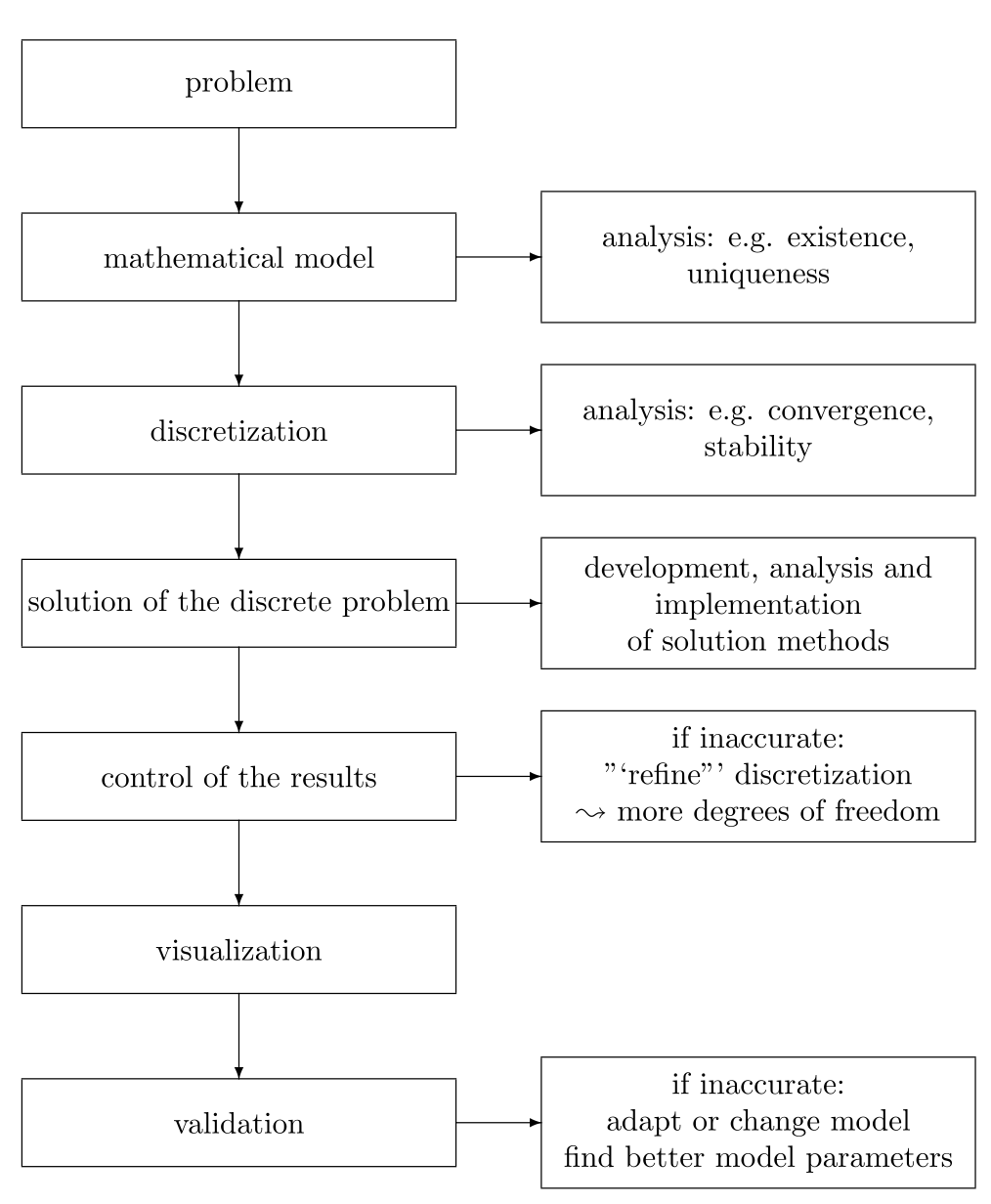
As possible error sources, we can identify
modeling errors,
errors in the given data,
wrong choice of solution method,
errors caused by the solution methods (or algorithms),
errors in the implementation,
...
In order to formalize the process \[\text{data}\quad\longrightarrow\quad \text{solving a problem}\quad\longrightarrow\quad \text{result}\] let us define \(X\) as the set of all possible data and \(Y\) as the set of all possible results. Then, the process of solving a problem means evaluating the “problem mapping” \[f\colon X\longrightarrow Y\] for given data \(x\in X.\) We denote by \(y=f(x)\) the solution of the problem \((f,x).\) The evaluation of the \(f\) will usually be done by means of an algorithm. In order to distinguish between the problem mapping \(f\) itself and the employed algorithm for evaluating \(f,\) we denote a solution or evaluation algorithm by \(\tilde{f}.\) This means we interpret our algorithm \(\tilde{f}\) as a somehow perturbed approximation to the original mapping \(f.\)
Let us emphasize that the choice of the algorithm \(\tilde{f}\) is not uniquely defined. In fact, it is one of the central aims of computational science to develop and analyze solution methods for a given problem (or a problem class), which combine as many desirable properties as possible; this might be efficiency, reliability, accuracy, a parallel design, or robustness with respect to changes in problem parameters.
Formally speaking, \(f(x)\) is the solution of \((f,x)\) for given exact data \(x\) and \(\tilde{f}(\tilde{x})\) the solution which has been obtained by applying the solution method or algorithm \(\tilde{f}\) to possibly perturbed data \(\tilde{x},\) see also 6.2. As a matter of fact, the exact solution \(f(x)\) in general is not available. Nevertheless, we need to quantify the quality of the actually computed solution \(\tilde{f}(\tilde{x})\) in order to decide whether \(\tilde{f}(\tilde{x})\) is an acceptable approximation of \(f(x)\) or not.
Since the set of real numbers \(\mathbb{R}\) is uncountable, we know that every approximation with a floating point system \(G(\beta,t,L,U)\) will lead to perturbations in the input data — regardless of whether the input data is exactly available or not.
As a first example, let us consider a mapping \(f\colon \mathbb{R}\longrightarrow\mathbb{R}.\) We try to estimate the influence of perturbations in the mapping \(f\) as follows: \[\begin{split} |f(x)-\tilde{f}(\tilde{x})| &= |f(x)-f(\tilde{x})+f(\tilde{x})-\tilde{f}(\tilde{x})| \\ &\le |f(x)-f(\tilde{x})| + |f(\tilde{x})-\tilde{f}(\tilde{x})|. \end{split}\] In the first line, we have added the term \(0=-f(\tilde{x})+f(\tilde{x}).\) This allows us to use the triangle inequality in order to get the final estimate. It furthermore adds the term \(f(\tilde{x}),\) which was not present before. By means of this term, we can now distinguish between perturbations in \(f\) and perturbations in \(x,\) and we can separate both using the triangle inequality.
The term \(|f(x)-f(\tilde{x})|\) is the unavoidable error caused by errors in the problem data \(x.\) Strongly connected to this error is the so-called condition number, which will be introduced in the next chapter. The second term \(|f(\tilde{x})-\tilde{f}(\tilde{x})|\) measures the additional errors introduced by the algorithm \(\tilde{f}.\) Investigating this term will lead us to the concept of stability of numerical algorithms.
6.2 Absolute and Relative Error
For measuring the error of an approximation \(\tilde{x}\) to \(x,\) we can simply look at the distance between the two, i.e. at the absolute error \[\epsilon_{\mathrm{abs}} = |x-\tilde{x}|\, .\] A “large” or “small” absolute error, in general, does not provide much information on the quality of the approximation \(\tilde{x}.\) For example, consider \(x=1.\) Then, \(x=-9\) seems to be a bad approximation to \(x.\) However, for \(y=10^9,\) \(\tilde{y}=10^9-10\) seems to be a good approximation, although both approximations have the same absolute error \(|x-\tilde{x}| = |y-\tilde{y}| = 10\)!
We therefore put the absolute error in relation to the size of \(x\) and define for \(x\not = 0\) the relative error \[\epsilon_{\mathrm{rel}} = \frac{|x-\tilde{x}|}{|x|}\, .\] Taking our example from above, we would arrive at a relative error of the approximation \(\tilde{x}\) to \(x\) of \(10\) and a relative error of the approximation \(\tilde{y}\) to \(y\) of \(10^{-8},\) which sounds more reasonable.
Looking at a certain problem \((f,x),\) we now would like to understand in which way errors or perturbations are propagated by means of \(f\) at the point \(x.\) Do errors get larger or smaller, or do they just remain?
We start with the absolute error. Let us assume that for our problem mapping \(f\) we can find a constant \(L_{\mathrm{abs}}\geq 0\) such that \[\tag{6.1} |f(x)- f(\tilde{x})| \leq L_{\mathrm{abs}} |x-\tilde{x}|\] for all \(x,\tilde{x}\in X.\)
If we interpret \(\delta x=\tilde{x}-x\) as perturbation \(\delta x,\) the above equation says that after applying the problem mapping \(f,\) the size of the perturbation \(|\delta x|\) is simply scaled by the factor \(L_{\mathrm{abs}}\) as follows \[|f(x)- f(x+\delta x)| \leq L_{\mathrm{abs}} |\delta x|\, .\] Dividing by \(|\delta x|\) for \(\delta x\not = 0,\) we see that \(L_{\mathrm{abs}}\) can alternatively be interpreted as an upper bound for the difference quotient \[\frac{|f(x)- f(x+\delta x)|}{ |\delta x|} \leq L_{\mathrm{abs}}\, .\]
Let us try to better understand this concept by looking at some examples. First, we consider the identity \(f(x)=x,\) \(x\in\mathbb{R}.\) Then, \(|f(x)- f(\tilde{x})| = |x-\tilde{x}|\leq 1\cdot |x-\tilde{x}|\) and we can choose \(L_{\mathrm{abs}} = 1.\) The identity is simply transporting perturbations without changing their size. They are conserved: neither enlarged nor reduced.
Now we consider the constant mapping \(f(x) = 1\) for all \(x\in \mathbb{R}.\) Then, \(|f(x)- f(\tilde{x})| =|1-1| = 0\) and we can choose \(L_{\mathrm{abs}}=0.\) The constant mapping is completely agnostic to perturbations, as it always gives the same response. All perturbations are removed — but also all information contained in the input data.
Exercise 6.1
Another simple mapping is \(f(x) = 5\cdot x.\) Which value would \(L_{\mathrm{abs}}\) have? Is \(f\) enlarging or reducing perturbations?
Analogously, we also can measure how the relative error is propagated, i.e. we look for \(L_{\mathrm{rel}}\geq 0\) such that \[\frac{|f(x)- f(\tilde{x})|}{|f(x)|} \leq L_{\mathrm{rel}} \frac{|x-\tilde{x}|}{|x|}\,\] for \(x, f(x) \not = 0\) and for all \(x,\tilde{x}\in \mathbb{R}.\)
In the next section, we will discuss this concept in more detail.
6.3 Condition Number and Well Posed Problems
Following Hadamard, we, therefore, will call a problem well-posed if small perturbations of the input data will cause only small changes in the solution. We will call a problem ill-posed if it is not well-posed.
Definition 6.1 • well-posed problem
The problem \((f,x)\) is called well-posed in \(B_\delta(x)\) if a constant \(L_{\text{abs}}\ge0\) exists such that \[\tag{6.2} |f(x)-f(\tilde{x})| \le L_{ \mathrm{abs}}|x-\tilde{x}| \quad\text{ for all }\tilde{x}\in B_\delta(x).\] If no such \(L_{\mathrm{abs}}\) exists, we call \((f,x)\) ill-posed in \(B_{\delta}(x).\)
For well-posed \((f,x),\) let \(L_{\mathrm{abs}}(\delta)\) denote the smallest constant with (6.2). If furthermore \(x\neq0\) and \(f(x)\neq0,\) let \(L_{\mathrm{rel}}(\delta)\) be the smallest constant \(L_{\mathrm{rel}}\) with \[\tag{6.3} \frac{|f(x)-f(\tilde{x})|}{|f(x)|}\le L_{\mathrm{rel}}\frac{|x-\tilde{x}|}{|x|} \quad\text{ for all }\tilde{x}\in B_\delta(x).\]
Remark 6.1
Condition is a local concept. The condition number will, in general, depend on the point \(x.\) Only for certain mappings, such as linear mappings, will a single global constant be sufficient.
The constants \(L_{\mathrm{abs}}(\delta)\) and \(L_{\mathrm{rel}}(\delta)\) measure locally around \(x\) how small perturbations \(\delta x\) of the input data through \(f\) are propagated. The measurement is done in the absolute or the relative error, respectively.
The mapping \(f\) does not have to be defined for all \(x\in X,\) but only on the (open) subset \(U\subset B_\delta(x).\)
Example 6.1
We start with some simple examples:
The constant mapping \(f: {\mathbb R}\to {\mathbb R}, f(x) := 0\) is clearly well-posed. It is even “destroying” information. In general, a very small condition number will give rise to small changes in the output, even for large changes in the input.
The linear mapping \(f: {\mathbb R}\to {\mathbb R}, f(x) := ax,\) \(0\not=a\in\mathbb{R}\) is also well-posed for each \(x\in\mathbb{R}.\) Obviously, we have \(L_{\mathrm{abs}} = |a|.\)
Exercise 6.2
The problem \(f: {\mathbb R}\to {\mathbb R}, f(x) := \sqrt{|x|}\) is ill-posed at \(x=0.\) In order to understand this argument better, plot the graph of \(f.\) What is happening to the tangent for \(|x| \ll 1\)?
Often, the term “forward problem” is connected to well-posed problems, whereas the term “backward problem” is connected to ill-posed problems.
We now define the condition number of a problem \((f,x)\):
Definition 6.2 • condition number
The absolute condition number of the problem \((f,x)\) is defined by \[\kappa_{\mathrm{abs}}=\lim\limits_{\delta\downarrow0}L_{\mathrm{abs}}(\delta).\] The relative condition number is defined by \[\kappa_{\mathrm{rel}}=\lim\limits_{\delta\downarrow0}L_{\mathrm{rel}}(\delta).\] A problem is called well-conditioned if \(\kappa\) is small, and ill-conditioned if \(\kappa\) is large.
The precise meaning of small or large in the above definition obviously depends on the problem. A problem with \(\kappa_{\mathrm{rel}}\le 1\) “forgets” or “destroys” information (in information theory, we would say “lossy compression” of input data, in the sense that we are not able to fully reconstruct the input from the output), which can be easily seen for \(f=\mathrm{const}.\)
6.2 illustrates the change in size of the “perturbation” ball around \(x,\) which is measured by means of the condition number.
From the definition, we have seen that the condition number will depend on \(f\) and the point \(x\) only. In particular, any algorithm for realising or approximating \(f\) is not considered in the definition of the condition number, and we can state
Remark 6.2
For differentiable \(f,\) here for simplicity \(f\colon\mathbb{R}\longrightarrow\mathbb{R},\) the condition numbers can be computed as follows \[\tag{6.4} \kappa_{\mathrm{abs}}=|f'(x)|\quad\text{and}\quad \kappa_{\mathrm{rel}}=\frac{|x|}{|f(x)|}|f'(x)|.\]
Exercise 6.3
Compute the condition number of the mappings \(f\colon \mathbb{R}\longrightarrow \mathbb{R}^+, f(x)=\exp(x),\) \(f\colon \mathbb{R}\longrightarrow \mathbb{R}^+, f(x)=x^2,\) \(f\colon \mathbb{R}^+\longrightarrow \mathbb{R}, f(x)=\ln(x).\) Compare the results. How does the respective condition number depend on \(x\)?
6.4 Condition of Elementary Operations
We would like to understand the behaviour of the elementary operations better. To this end, we investigate their respective condition.
6.4.0.0.1 Addition and Subtraction
We start with addition and subtraction.
Theorem 6.1
Let \(f\colon \mathbb{R}^2\to\mathbb{R}\) with \[\begin{pmatrix}a\\b\end{pmatrix}\mapsto f(a,b)=a+b\, .\] and let \(a,b\not= 0.\) Let \(\tilde{a},\tilde{b}\) be approximations of \(a\) and \(b,\) respectively. We assume that the relative error of these approximations is bounded by \(0<\delta_a,\delta_b\leq \delta,\) i.e. \[|a - \tilde{a}| \leq \delta_a |a| \mbox{ and } |b - \tilde{b}| \leq \delta_b |b| \, .\] Then, we can estimate the relative error in addition (and subtraction) \[\begin{aligned} \frac {|f(a,b)-f(\tilde{a},\tilde{b})|}{|f(a,b)|} &\leq& \frac {|a|+|b|}{|a+b|} \delta\, . \end{aligned}\]
Proof. Exercise.
Corollary 6.2 • Addition and Subtraction
Addition is well-conditioned and for the relative condition number \(\kappa_{\mathrm{rel}}\) of the addition it holds \(\kappa_{\mathrm{rel}}=1.\) Subtraction can be arbitrarily ill-conditioned, in particular, if the cancellation of leading digits occurs.
Proof. In the case of addition, i.e. if \(a\) and \(b\) have the same sign, \(\frac {|a|+|b|}{|a+b|}=1\) and we obtain \(\kappa_{\mathrm{rel}}=1.\)
In the case of subtraction, i.e. if \(a\) and \(b\) have a different sign, in general, we will have \(\frac {|a|+|b|}{|a+b|}\geq 1,\) as we can see from the triangle inequality. We then see that this term can become arbitrarily large if \(|a|\approx |b|.\) Assume, for example, \(b=-a+\epsilon\) with \(\epsilon>0\) small. Then \[\kappa_{\mathrm{rel}} = \frac {|a|+|b|}{|a+b|} = \frac {2|a|+\epsilon}{\epsilon} \geq \frac {2|a|}{\epsilon}\] and we can find for each \(C\in\mathbb{R}\) an \(\epsilon>0\) such that \(\kappa_{\mathrm{rel}} > C,\) i.e. the relative condition number of subtraction can be arbitrarily large.
Remark 6.3
Practical consequences are:
For addition, perturbations in the input data are simply transported. From the point of view of condition number, addition is your friend with \(\kappa_{\mathrm{rel}}=1\)!
Subtraction is arbitrarily ill-conditioned in the case of cancellation of leading digits. Thus, errors get enlarged. The subtraction of approximately equal numbers is to be avoided.
6.4.0.0.2 Leading Order Terms
Before doing so, we shortly have to introduce the concept of a leading order term. To this end, let us consider the polynomial \(p(x)= x^3-5x^2-x+7.\) As can be seen, for \(|x|\to\infty,\) the term which dominates all other terms is the term with the highest power, in this case \(x^3.\) For example, set \(x=1000.\) Then, \(|x^3| =10^9 \gg |5x^2| = 5\cdot 10^6 \gg |x|=1000 \gg 7.\) Thus, in order to investigate the qualitative behaviour of \(p(x)\) for \(|x|\to\infty,\) it is sufficient to look at the term \(x^3.\) Therefore, we call this term the leading term. The same concept can be applied for \(|x|\to 0.\) We have, however, to be careful, as for numbers \(|x| < 1,\) the term with the smallest exponent provides the largest contribution in absolute value. For example, consider the polynomial \(q(x)=x+x^2.\) Then, for \(0\leq x \ll 1,\) we will have \(x\gg x^2.\) For example, let \(x=1/2.\) Then \(x=1/2 > x^2=1/4,\) and for \(x=10^{-3}\) we see \(x=10^{-3} \gg x^2=10^{-9}.\) Thus, we see that for small \(|x|,\) the dominant term is the one with the lowest exponent. As a consequence, for \(0\leq x \ll 1,\) we can say that \(q(x)=x+x^2\) in leading order is equal to \(\tilde{q}(x) = x.\)
In order to formalize this idea, we make use of the Landau Symbol, see Definition 6.5, which is formally introduced in Equation (6.6). By setting \(g(x)=x\) in Equation (6.6), we see that we can write \[q(x) = o(x) \Leftrightarrow \lim_{x\to 0 } \frac{f(x)}{x} = 0\, .\]
6.4.0.0.3 Multiplication and Division
We now consider multiplication and division.
Theorem 6.3 • Multiplication and Division
Let \(f\colon \mathbb{R}^2\to\mathbb{R}\) with \[\begin{pmatrix}a\\b\end{pmatrix}\mapsto f(a,b)=a\cdot b\, .\] and let \(a,b\not= 0.\) Let \(\tilde{a},\tilde{b}\) be approximations of \(a\) and \(b,\) respectively, and let the relative error of these approximations be bounded with \(\delta>0\) \[\begin{aligned} |a - \tilde{a}| &\leq & \delta |a| \\ |b - \tilde{b}| &\leq & \delta |b| \, . \end{aligned}\] Then, the condition of multiplication in leading order is \(\kappa_{\mathrm{rel}}=2.\)
Proof. Exercise.
6.5 Landau Symbols
Definition 6.3
Let \(f , g \colon (a, \infty ) \longrightarrow R.\) Then we write symbolically \[f(x) = o(g(x)) \text{ for } x \to\infty\, ,\] (we say \(f (x)\) equals small-oh of \(g(x)\)) if for every \(\epsilon >0\) there exists \(R > a\) such that \[|f (x)| \leq \epsilon |g(x)| \text{ for all } x \geq R \, .\] Let \(D\subset \mathbb{R}\) and \(f,g\colon D\longrightarrow \mathbb{R}.\) We write \[\tag{6.6} f(x) =o(g(x)) \text{ for } x\to x_0\, , x \in D\,,\] if for every \(\epsilon> 0\) there is a \(\delta >0\) such that \(|f(x)|\leq \epsilon |g(x)|\) for all \(x\in D\) with \(|x-x_0|<\delta.\)
For us, the second part of the definition is more interesting, as we use the Landau symbol typically for local approximations. We note that for \(g(x)\not= 0\) Equation (6.6) means that \[\lim_{\stackrel{x\to x_0}{x\in D}} \frac{f(x)}{g(x)} = 0\, .\] That means that \(f\) tends “faster” to \(0\) than \(g.\) For example, consider \(f(x)=x^2\) and \(g(x)=x,\) we get \(\frac{f(x)}{g(x)}=x \to 0\) for \(x\to 0.\)
Exercise 6.4
Let \(x_0 =0,\) \(a,b\in\mathbb{R}\) arbitrary but fixed and let \(f(x) = a\cdot x^p\) with \(p>0.\) For which \(q>0\) does it hold for \(g(x)= b \cdot x^q\) that \(f(x) = o(g(x))\) for \(x\to x_0\)? Hint: a) We already have considered the case \(p=2, q=1\) above. b) Make sure to cover the special case \(a=0\) and \(b=0\) in your considerations.