4 Numbers and Floating Point Numbers
4.1 Representation of Numbers
We usually represent numbers in the decimal system. For example, the number \(273\) we interpret as \[\begin{aligned} 273 &=& 2\cdot 100 + 7\cdot 10 + 3\cdot 1\\ & = & 2\cdot 10^2 + 7\cdot 10^1 + 3\cdot 10^0 \, . \end{aligned}\] Therefore, we talk about a decimal representation, as numbers are expressed in multiples of powers of \(10.\) However, looking at the above number, we see that we could also write it as \[\begin{aligned} 273 & = & 256 + 16 + 1 \\ & = & 1 \cdot 2^8 + 1 \cdot 2^4 + 1 \cdot 2^0 \\ & = & 1 \cdot 2^8 + 0 \cdot 2^7 + 0 \cdot 2^6 + 0 \cdot 2^5 + 1 \cdot 2^4 + 0 \cdot 2^3 1 + 0 \cdot 2^2 + 0 \cdot 2^1 +1 \cdot 2^0 \end{aligned}\] i.e. using powers of two. Thus, we see that the decimal number \((273)_{10},\) where the subscript \({}_{10}\) indicates that this number is to be interpreted with respect to the basis \(10,\) can equally be represented as the binary number \((100010001)_{2}.\)
Definition 4.1
An alphabet \(\Sigma\) is a finite ordered set. The elements of \(\Sigma\) are called letters. Furthermore, we denote by \(\Sigma^*\) the set of all finite words over A, i.e. the set of finite concatenations of letters from \(\Sigma.\)
Furthermore, for every natural number \(b>0,\) we define \[\Sigma_b =\{0,1,\ldots,b-1\}\] to be the alphabet of the \(b\)-adic (number) system. We call \(b\) the basis of the \(b\)-adic system.
Example 4.1
As a first example, we can consider the alphabet we are using for the decimal system, i.e. \[\Sigma_{10} = \{0,1,2,3,4,5,6,7,8,9\} \, .\] Then, \(\text{``}273\text{''}\in \Sigma^*\) is a word over \(\Sigma.\) Other alphabets are
\(\Sigma_2 = \{0,1\},\) the dual or binary alphabet
\(\Sigma_8 = \{0,1,2,3,4,5,6,7\},\) the octal alphabet
\(\Sigma_{16} = \{0,1,2,3,4,5,6,7,8,9,A,B,C,D,E,F\},\) the hexadecimal alphabet
We now investigate how natural numbers can be represented in a \(b\)-adic system.
Theorem 4.1
Let \(b, n\in \mathbb{N}\) and let \(b>1.\) Then, every number \(z\in \mathbb{N}\) with \(0\leq z\leq b^n-1\) can uniquely be represented as a word of length \(n\) over \(\Sigma_b\) with \[z = \sum_{i=0}^{n-1} z_i b^i \, .\] Here, \(z_i\in\Sigma_b\) for \(i=0,\ldots,n-1\)
The proof is carried out via induction. For the proof we will need the floor and ceiling functions (Gaussian brackets) which are defined for \(x\in\mathbb{R}\) as \[\begin{aligned}
\lfloor x\rfloor &=& \max \{k\in\mathbb{Z}\colon k\leq x\}\\
\lceil x\rceil &=& \min \{k\in\mathbb{Z}\colon k\geq x\}
\end{aligned}\] as well as the modulo operation mod defined for \(x\in\mathbb{Z}\) and \(y\in \mathbb{N}\setminus\{0\}\) as \[x\mod y = x-y\cdot \left\lfloor \frac{x}{y}\right\rfloor\, .\] From the above definitions, it follows that for \(z\in\mathbb{N}\) we have \[z=\lfloor z/b\rfloor\cdot b + (z \mod b)\, .\]
Example 4.2
The operation of the Gaussian brackets and of \(mod\) can be easily understood by inserting some numbers
\(\lfloor 13.2\rfloor = 13\)
\(23 \mod 6 = 23 - 6 \lfloor \frac{23}{6}\rfloor = 23 - 6\cdot3 = 5\)
\(23 = \lfloor 23/6\rfloor\cdot 6 + (23 \mod 6)\ = 3\cdot 6 + 5\)
Proof. A (\(n=1\)) For \(z\in \mathbb{N}\) with \(0\leq z < b\) we can uniquely represent \(z\) as \(z = \sum_{i=0}^{n-1} z_i b^i\) with \(z_0=z\) and \(z_i=0\) else.
B (\(n\to n+1\)) We assume that every number \(\hat{z}\) with \(0\leq \hat{z} < z\) can be represented as \(\hat{z} = \sum_{i=0}^{n-1} \hat{z}_i b^i\) with \(\hat z_i\in\Sigma_b\) for \(i=0,1,\ldots,n-1.\)
We first note that we have \(z=\lfloor z/b\rfloor\cdot b + (z \mod b).\) We now set \(\hat{z} = \lfloor z/b\rfloor.\) Then, we have \(\hat{z} < z,\) since \(b>1.\) By the above assumption, \(\hat{z}\) has the representation \(\hat{z} = \sum_{i=0}^{n-1} \hat{z}_i b^i\) with \(\hat z_i\in\Sigma_b\) for \(i=0,1,\ldots,n-1.\) Due to \(\hat z\cdot b \leq z \leq b^n-1\) we get \(\hat z_{n-1}=0.\) This leads to \[\begin{aligned} z= \hat z\cdot b + (z \mod b) & = & b\cdot \sum_{i=0}^{n-2} \hat{z}_i b^i + (z \mod b) \\ & = & \sum_{i=1}^{n-1} \hat{z}_{i-1} b^i + (z \mod b) \\ & = & \sum_{i=0}^{n-1} z_{i} b^i \, , \end{aligned}\] with \(z_0= z\mod b\) and \(z_i = \hat{z}_{i-1}\) for \(i=1,2,\ldots,n-1\) .
We now show that this representation is unique. Let us assume that \(z_0\in \mathbb{N}\) has two different representations \[z = \sum_{i=0}^{n-1} z_i b^i = \sum_{i=0}^{n-1} \hat{z}_i b^i\, .\] Let \(m=\max\{i\colon 0\leq i\leq n-1 \mbox{ with } z_i\not = \hat z_i \}.\) For \(0\leq i\leq n-1\) we have \(z_i\geq 0\) and \(\hat z_i\leq b-1.\) This implies \(z_i -\hat z_i\geq 1-b.\) Without loss of generality, let \(z_m > \hat z_m.\) This implies \[\begin{aligned} 0 & = & z - z = \sum_{i=0}^{m} z_{i} b^i - \sum_{i=0}^{m}\hat z_{i} b^i\\ & =& \sum_{i=0}^{m} (z_{i}-\hat z_i) b^i\\ &\geq& b^m + \sum_{i=0}^{m-1} (1-b) b^i\\ &=& b^m + \sum_{i=0}^{m-1} b^i - \sum_{i=0}^{m-1} b^{i+1} = b^m + b^0-b^m\\ & = & 1\, .\\ \end{aligned}\] Consequently, the representation is unique.
Remark 4.1
Some remarks concerning the above definitions:
for every \(n \in N\) an index \(i > n\) exists such that \(x_i\) is not equal to \(b-1\). We know that \(0.9999999..... = 1\) (or will know once we will have learned about the convergence of infinite series). Thus, there are two representations for \(1.\) But we want uniqueness. As the argument will also apply to numbers such as \(0.156784999999999...,\) we have to exclude a constant sequence of \(9\)’s (i.e. \((b-1)\)’s). If you would require only that there exists an \(i>0\) with \(x_i\not= b_{i-1},\) after this \(i\) there could still be infinitely many \((b-1)\)’s. So we require that, regardless of the position at which we enter the sequence of digits (and this entrance point is \(n\)), we will find a number different from \(b_i-1\) afterwards (which is your \(i\)).
The \(b\)-adic representation is valid for every number different from \(0.\) The number \(0\) is simply represented as zero.
4.2 Floating Point Representation and Machine Accuracy
Computers are predominantly based on numbers systems with basis \(b=2.\) We therefore consider the representation of integers in a computer using bits \(d\in \{0,1\}.\)
4.2.1 Integers
For representing an integer \(z\in\mathbb{Z}\) we use \(N\) bits, i.e. \[z \hat{=} d_{N-1}d_{N-2}\cdots d_0\quad\text{ with }d_i\in\{0,1\}.\] That means \[\tag{4.2}
z = d_0+d_1 2^1 + d_2 2^2 + \ldots + d_{N-1} 2^{N-1}.\] Natural numbers are represented as unsigned integers; integers additionally have one bit for the sign \(s\in\{0,1\}.\) That means \[z \hat{=} s|d_{N-2}d_{N-3}\cdots d_0
\hat{=} (-1)^s\sum\limits_{i=0}^{N-2}d_i2^i.\]
Example 4.3
Let \(N=4.\) Then we have the first unsigned integers \[\begin{aligned} 0&\hat{=}&0000,\\ 1&\hat{=}&0001,\\ 2&\hat{=}&0010,\\ 3&\hat{=}&0011. \end{aligned}\]
In the case of the above integer representation, zero is not represented uniquely; moreover, subtraction cannot be treated the same way as addition. Thus, for negative numbers, we use the following representation as two’s complement \[1|d_{N-2}\ldots d_0\hat{=}-\left(1+\sum\limits_{i=0}^{N-2}(1-d_i)2^i\right) \, .\] For subtraction, each \(z<0\) is represented as above. Then all bits are changed and finally \(1\) is added.
Example 4.4
Let \(N=4.\) Then we have \[-3\hat{=}-011\hat{=}1|101.\]
For given \(N,\) we can represent integers within the following range \[z_{\text{min}}= -2^{N-1}=-\left(1+\sum\limits_{i=0}^{N-2}1\cdot2^i\right) \leq z \leq \sum\limits_{i=0}^{N-2}1\cdot2^i=2^{N-1}-1=z_{\text{max}}\] Usually \(N = 32\) is called integer and \(N=64\) long integer. Numbers \(z\) with \(z<z_{\text{min}}\) or \(z>z_{\text{max}}\) lead to underflow or overflow, respectively.
4.2.2
The representation of integers within the admissible range is exact. For real numbers, this is not possible.
Remark 4.2
Computer algebra programs as Maple or Mathematica can manipulate formulas and certain expressions. This is, however, not “exact” floating point arithmetic.
We use an approximate representation of real numbers. Thereby, we aim for
a small rounding error
a huge range of numbers, which can be represented
stability of the elementary operations \(\{+,-,\cdot,/\}\)
We now have two possibilities: We can approximate a real number \(x\in\mathbb{R}\) with a floating point number \(\text{rd}(x)\) such that either the absolute error is bounded by some \(\varepsilon > 0,\) i.e. \[|x-\text{rd}(x)|\leq\varepsilon,\] or such that the relative error is bounded: \[|x-\text{rd}(x)|\leq\varepsilon|x|\, .\] We choose the relative error, since it is in general the appropriate error measure and since this choice allows for a much larger range of representable numbers.
Definition 4.2 • floating point numbers
Let a basis \(\beta\in\mathbb{N}\) with \(\beta\ge2\) be given and furthermore a range \([L,U]\cap\mathbb{Z}\) of representable exponents and the length of the mantissa \(t\in\mathbb{N}.\) If a number \(\tilde{x}\in\mathbb{R}\) can be represented in the form \[\tag{4.4} \tilde{x}=(-1)^sa\beta^e\] where \(s\in\{0,1\}\) is the sign bit, \(e\in[L,U]\cap\mathbb{Z}\) the exponent and \(a=\sum_{i=0}^t a_i\beta^{-i}\) with \(a_i=0,\ldots, \beta-1,\) \(a_0\neq0,\) we call \(\tilde{x}\) floating point number. Since \(a_0\neq 0,\) we call (4.4) normalized floating point representation. We denote the set of floating point numbers defined by \(\beta, t, [L,U]\) by \({\mathcal G}\) or \({\mathcal G}(\beta, t, [L, U])\) (floating point format).
Remark 4.3
If \(\beta=2,\) we will have \(a_i\in\{0,1\}.\) In this case, for the normalized representation the leading bit always has the value \(1.\) This leads to \[a=\sum_{i=0}^t a_i 2^{-i} = 1 + \sum_{i=1}^t a_i 2^{-i} = 1 + m\, .\] Thus, we have “saved” one bit when storing the floating point number. If the leading bit is not set, we have a denormalized floating point representation. Then, however, the mantissa is also one bit shorter.
In case \(\hat{x}\in{\mathcal G}\) does not have a unique representation, i.e. \(\hat{x}=a\beta^e=A\beta^E,\) we clearly have \(A=a\beta^j\) and \(E=e-j.\) We thus assume \(\beta^{-1}\leq a<1,\) which gives the desired uniqueness. For fixed \(\beta,t,[L, U],\) the set of all representable floating point numbers is clearly much smaller than \(\mathbb{R}.\) Thus, we cannot represent all real numbers.
The range of representable numbers is given by \[x_{\min} \leq |\tilde{x}| \leq x_{\max}\] where we have \[\begin{aligned} x_{\min} & = & \frac{1}{\beta}\cdot \beta^{L} = \beta^{L-1} \\ x_{\max} & = & (\beta-1) \left(1 + \beta^{-1} + \beta^{-2} + ... + \beta^{-t} \right)\beta^{U} = (\beta-\beta^{-t}) \beta^{U} \end{aligned}\]
Theorem 4.2
Let \(\beta\) be a multiple of \(2.\) Then, for each number \(x\in[L,U],\) there exists a floating point number \(\text{rd}(x),\) \({\mathcal G}(\beta,t, [L,U])\) with relative error \[\frac{|x-\text{rd}(x)|}{|x|}\leq\frac{1}{2} \beta^{-(t-1)}=:\mathrm{eps}.\]
The proof may be carried out as an exercise.
Remark 4.4
The number \(\mathrm{eps}\) is called machine accuracy and bounds the relative error of the floating point representation. Each floating point number thus represents an interval in \(\mathbb{R}\) (at least in case of the normalized representation). As a consequence, a (relative) error of \(\mathrm{eps}\) in the given data is unavoidable. This also holds true if the given data seems to be “exactly representable”, e.g. \(x=1,2,\frac 12.\)
Example 4.5
For \(\beta=10\) we have \[5\hat{=}0.5 \cdot 10^1 \hat{=} 0.50\ldots0\] and \[50 \hat{=} 0.5\cdot 10^2\, .\]
By means of the mapping \(\text{rd}: [x_{\min},x_{\max}]\longrightarrow {\mathcal G},\) each \(x\in\mathbb{R}\) gets assigned one and only one floating point number. We moreover have \(\text{rd}\circ\text{rd}=\text{rd},\) i.e. \(\text{rd}\) is a projection. We call the number \(\text{rd}(x)\) floating point representation of \(x.\) What does \(1\)% error mean? It means, there exists \(\tilde{x}\) with \[\frac{|x-\tilde{x}|}{|x|}\leq \frac{1}{100}\, .\]
The mapping \(\text{rd}\) is not injective. Several different numbers will be rounded to the same floating point number. Computing in \({\mathcal G}\) is computing with intervals: each floating point number \(\tilde{x}\) represents an interval around \(\tilde{x}\) (the size of the interval can vary with \(x\)). We set \[x\stackrel{{\mathcal G}}{=}y:\iff x\tilde{=}y:\iff \text{rd}(x)=\text{rd}(y).\] As a consequence, within source code statements such as x==y should never be used. Instead, \(|x-y|\leq r\) should be taken, where \(r\) is suitably choosen (e.g. \(r=\mathrm{eps}\cdot |x|\)). Let us finally note that in the denormalized floating point representation the relative error is not bounded by \(\mathrm{eps}\) any more.
The IEEE-standard (IEEE : Institute of Electrical and Electronics Engineers) specifies the data types float and double as follows:
| sign | exponent | mantissa | bias | |
|---|---|---|---|---|
| \(32\) bit (float) | \(1(31)\) | \(8(30-23)\) | \(23(22-0)\) | \(127\) |
| \(64\) bit (double) | \(1(63)\) | \(11(62-52)\) | \(52(51-0)\) | \(1023\) |
We call the \(32\)-bit number float (single precision), and the \(64\)-bit number double (double precision).
For double, this leads —taking into account the hidden bit— to \(\mathrm{eps}=\frac{1}{2} 2^{-52}=2^{-53}\approx 1.1 \cdot 10^{-16}.\) Often, for the machine accuracy \(\hat{\mathrm{eps}}_{\text{double}}=2.2 \cdot 10^{-16}
=2\cdot \mathrm{eps}\) can be found. This does not correspond to the definition given here.
Remark 4.5
In the IEEE 754 standard, a normalized floating point number must have at least one “1” in the exponent bits.
Remark 4.6
In order to get the actual value of the exponent, the (positive) bias has to be subtracted from the stored value. This ensures that the stored value is always non-negative, which makes the comparison of exponents easier than it would be in a two-complement representation. The exponents \(128(\hat{=}1111 1111)\) and \(-127(\hat{=}0000 0000)\) are reserved. If the exponent consists only of ones and if the
mantissa is \(0,\) the represented number is \(\pm\) infinity
mantissa is \(100 \ldots 0,\) the represented number is not defined (e.g. \(0\cdot\infty\))
mantissa is \(0\ast\) and \(s=1,\) we have the case NaN (not a number).
Denormalizing for exponent \(0\) reduces the accuracy but allows for representing very small numbers and \(0.\) The IEEE-Standard 754 has \(a_0\neq0\) instead of \(a_1\neq0,\) i.e. \(1.0 \cdot 2^{-1}\) instead of \(0.1 \cdot 2^0.\)
4.2.3 Floating Point Arithmetic and Cancellation of Leading Digits
Ideally, when doing computations in floating point arithmetic, the relative error of the result of one of the elementary operations \(\{+,-,\cdot,/\}\) should be bounded by the machine accuracy. Let us therefore start with the following
Definition 4.3
Let \(\ast\in\{+,-,\cdot,/\}.\) Then we define the floating point operation \(\hat{\ast}\) by \(x\hat{\ast}y:=\text{rd}(x\ast y).\)
Remark 4.7
Usually, this is realized by computing internally with higher accuracy.
Corollary 4.3
For all floating point numbers we have \(x\hat{\ast}y=(x\ast y)(1+\varepsilon)\) with \(|\varepsilon|\leq\mathrm{eps},\) if the result is in \({\mathcal G}.\)
Remark 4.8
In general, floating point operations are not associative, i.e. \[( x \hat{+} y ) \hat{+} z \neq x \hat{+} ( y \hat{+} z ).\] For example, consider \(\beta=10, L=-9, U=9, t=1\) and set \(x=0.1 \cdot 10^1, y=-0.1\cdot 10^1\) and \(z=0.1\cdot 10^{-1}.\)
We now investigate the influence of relative errors on the elementary operations. We start with the addition. Let \(x,y\) be floating point numbers. Then, \(x+y\) can have a mantissa with length \(>t.\) For example, let \(\beta=10, L=-9, U=9\) and \(t=2.\) Then we have \[0.10 \cdot 10^0 + 0.10 \cdot 10^2 = 0.101 \cdot 10^2\,\hat{=}\, 0.10\cdot 10^2\,.\] Due to \(t=2,\) on the right hand side information is destroyed. In case of \[0.51 \cdot 10^9 + 0.5 \cdot 10^9 = 0.101\cdot 10^{10}\hat{=} 0.1 \cdot 10^{10}\notin{\mathcal G}\] we find an overflow in the exponent. An underflow in the exponent results from \[0.51 \cdot 10^{-9} - 0.5 \cdot 10^{-9} = 0.10 \cdot 10^{-10} \notin{\mathcal G}.\]
4.2.4 Cancellation of leading digits
The subtraction of approximately equal numbers in a floating point system can lead to unwanted consequences in terms of accuracy. We illustrate this with the following two examples:
Let \[\begin{aligned} a&=&0.123467\!\ast\\ b&=&0.123456\ast \end{aligned}\] be given. Both numbers might be disturbed at the 7th digit. Then, we have \[a-b=0.000011\ast=0.11\!\ast\cdot10^{-4}.\] An error in the data in the 7th digit leads to an error in the result in the 3rd digit. This means \(\kappa_{\text{rel}}\approx10^{4}.\)
Consider the polynomial \[f(x,y)=(x-2y)^3=x^3-6x^2y+12xy^2-8y^3\] for \(x=10 000 000,\ y=4 999 999.\) We have \[\begin{aligned} a&:=&x^3+12xy^2\approx3.9999000001202585\cdot10^{21}\\ b&:=&8y^3+6x^2y\approx3.9999000001973427\cdot10^{21} \end{aligned}\] and, in floating point arithmetic (double), \[a-b = 524.388.\] For \(\mathrm{eps}\approx 1\cdot 10^{-16}\) the error is increased as follows: \[\kappa_{\text{rel}}=\frac{a+b}{|a-b|}\approx \frac{8\cdot10^{21}}2=4\cdot10^{21} \, .\]
As a consequence we see that the subtraction of approximately equal numbers should be avoided. If it is unavoidable, it should be carried out at the beginning of an algorithm.
Example 4.6
Employing the \(pq\)-formula for solving the quadratic equation \[x^2 + px + q = 0\] we have for the case \(p^2\ge4 q\) (this ensures a real solution) \[x_{1/2}=-\frac{p}{2}\pm\sqrt{\left(\frac{p}{2}\right)^2-q}.\] If \(p\gg q,\) cancellation of leading digits occurs. One possibility to avoid this is to compute first the solution \(x_1\) with larger absolute value. Then, following Vieta’s theorem, we can compute the missing solution as \(x_2=q/x_1.\)
4.2.5 Special Numbers and their Representation
Certain operations will not lead to a floating point number but to a so called “exception”. We might encounter overflow or underflow, or division by \(0\) might occur. In these cases, special numbers will be returned to the programmer.
4.2.6 Summation Techniques
We would like to illustrate that the floating point addition \(\hat{+}\) in general is not associative.
We consider infinite series \[1+\sum\limits_{k=2}^\infty \frac {1}{k} = 1+ \frac{1}{2} +\frac{1}{3} +\cdots \, ,\] which is called harmonic series. The harmonic series is said to converge iff the sequence \((S_K)_{K\in \mathbb{N}}\) of the so called partial sums \[S_K=\sum\limits_{k=2}^{K} \frac {1}{k}\] converges. Since the harmonic series is divergent (as you will see in Calculus 1), also the sequence \((S_K)\) of the partial sums diverges. However, in floating point arithmetic we expect the summation to stall at a certain point, as the sequence \(x_k=\frac{1}{k}\) converges to \(0.\) In order to investigate this, we compute the \(2^m\)–th partial sum, \(m>0\) of the above series, i.e. \[S_{2^m}=1+\sum\limits_{k=2}^{2^m} \frac {1}{k}\, .\] For doing so, we use three different summation techniques.
The first technique is the intuitive forward summation:
fwd = 1;
for k=2:n
 fwd = fwd + 1/k;
end
The second technique is backward summation:
n = 2^fix(m);
bwd = 0;
for k=n:-1:2
 bwd = bwd + 1/k;
end
bwd = bwd + 1;
The third technique is the so called hierarchical summation.
n = 2^fix(m);
a1 = 0;
a2 = 0;
I=[3:2:n];
n = n/2;
sum = zeros(1,n);
sum(1) = 1 + 1/2;
for k=I
a1 = 1/k;
a2 = 1/(k+1);
sum(1+(k-1)/2) = a1+a2;
end
while(n > 2)
for i=1:2:n
sum(i) = sum(k)+sum(k+1);
end
sum = sum([1:2:n]);
n = n/2;
end
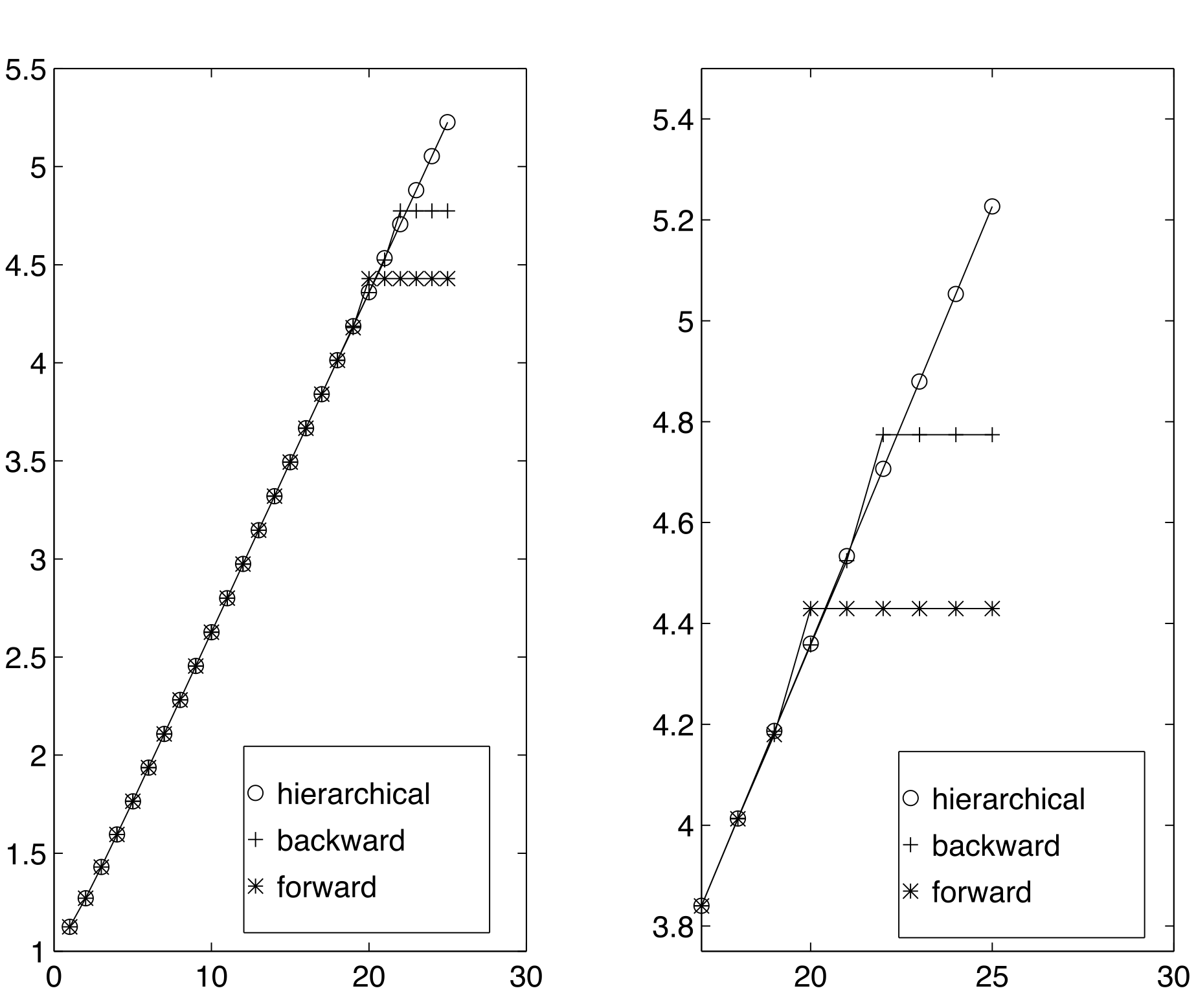
hier = sum(1)+sum(2); We illustrate the hierarchic summation for \(K=8.\) We have \[\begin{aligned} S_8 &= x_1+ \cdots + x_8 \\ & = (\underbrace{(x_1+x_2)}_{=s_{1,2}}+\underbrace{(x_3+x_4)}_{=s_{3,4}} + \underbrace{(x_5+x_6)}_{=s_{5,6}}+\underbrace{(x_7+x_8)}_{=s_{7,8}}) \\ & = \underbrace{(s_{1,2}+s_{3,4})}_{=s_{1,2,3,4}} +\underbrace{(s_{5,6}+s_{7,8})}_{=s_{5,6,7,8}}\\ & = s_{1,2,3,4} + s_{5,6,7,8} \, . \end{aligned}\] Figure 4.1 shows a comparison of the three different approaches. As can be seen, the summation stalls already very relatively small values of the partial sums, as for the individual contributions \(1/k\) it also holds \(1/k\to 0\) for \(k\to\infty.\) The best results are achieved for the hierarchical summation.